QGIS joining data
8.9 Load data
- Search for and open QGIS
- Click on the open data source manager. Just above the word browser in the top left of the screen
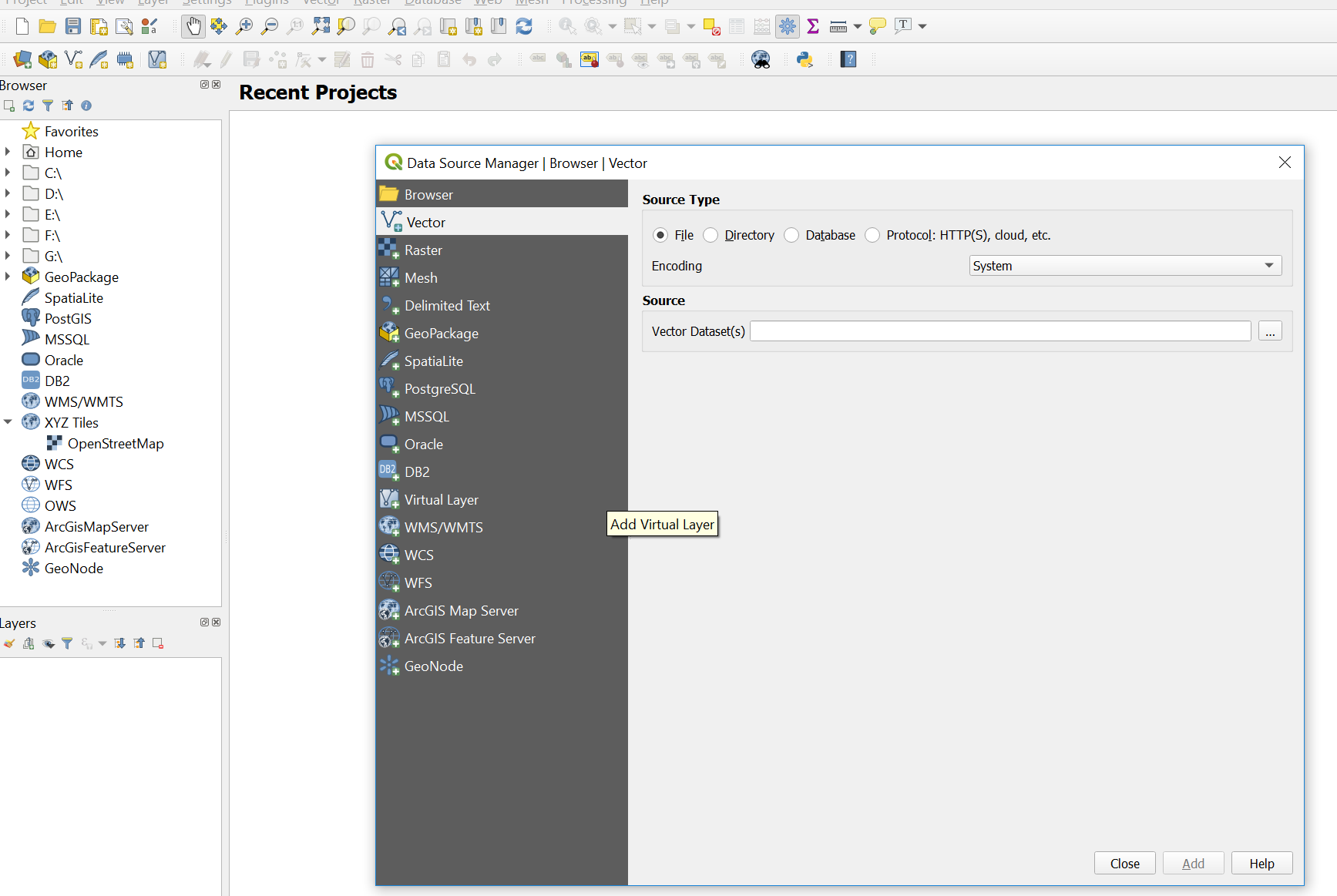
- Navigate to the
London_Borough_Excluding_MHW.shpand add it, you then have to close the data source manager.
You can right click on the layer to view the attribute table, however the .csv file must be loaded into QGIS in order to join it to a shapefile.
- Open the data source manager and select Delimited Text
- Navigate to our
.csvfile and provide a suitable layer name - Under Record and Fields Options make sure the number of header lines to discard is 0 and the First record has field names box is selected (this is assuming you left a title for each column in your
.csv) - Under Geometry Definition select No geometry (attribute table only)
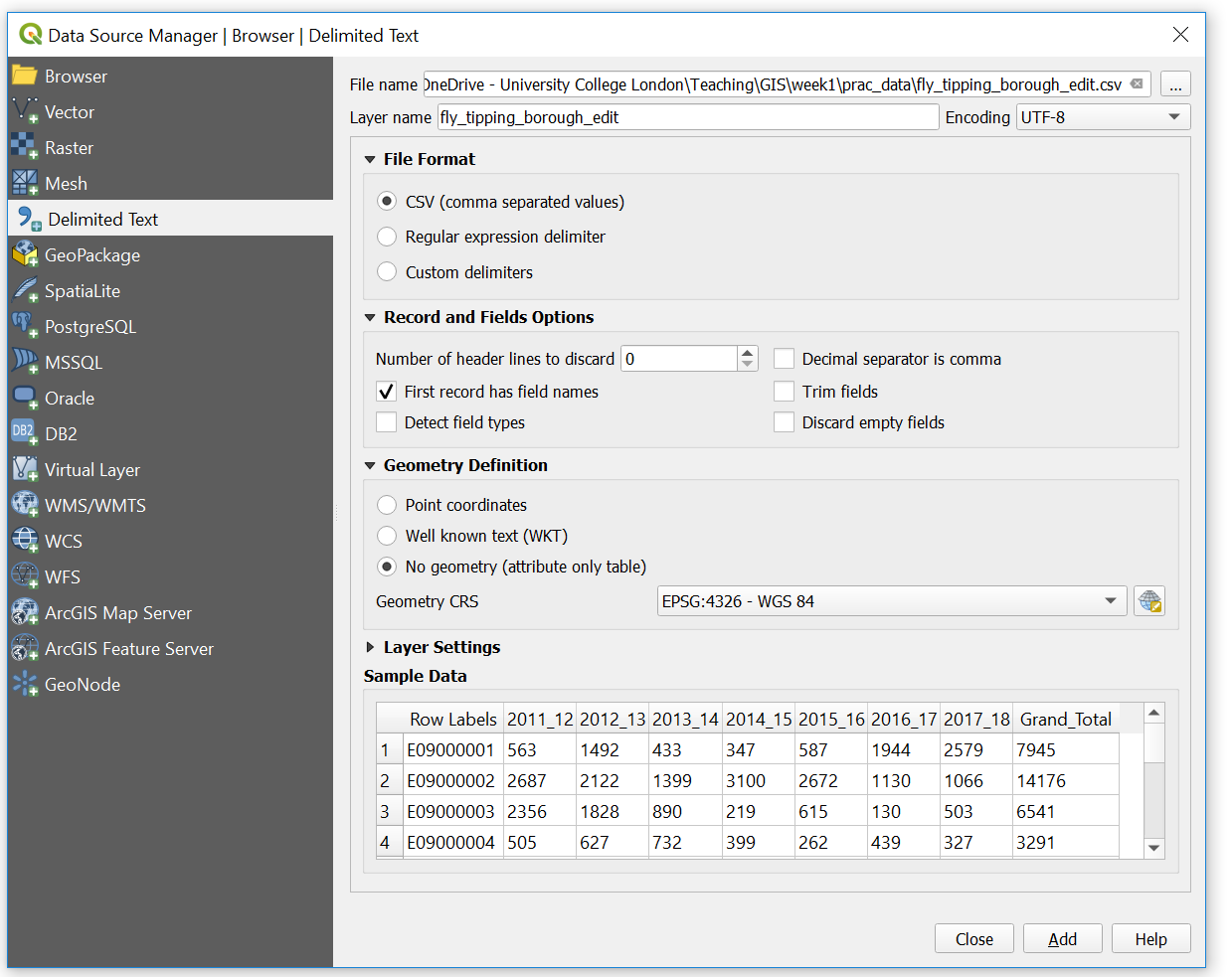
Does the sample data seem right?
- If so, click add then close
Note Your .csv might have a extra header present (a row before Row Labels). You can either: (a) close this and go and delete this in the .csv now and reload it or (b) change the number of header lines to discard to 1 in the Record and Fields Options in the screenshot above.
8.10 Join data
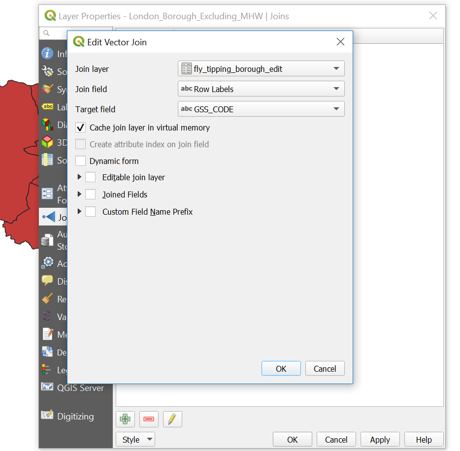
- Right click on the London boroughs layer > Properties > Joins
- Click the plus button at the bottom of the box
- Complete the dialogue box
8.11 Export data
Now let’s export to a GeoPackage.
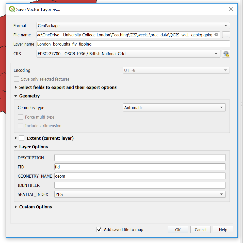
- Right click on the London boroughs layer > Export > Save Feature As
- Select the GeoPackage format and complete the File name (the saved file name for the GeoPackage) and the Layer name (the name for this layer within the GeoPackage). Recall that a GeoPackage can store many data layers as a single file
- The new layer will be added to the map, so you can remove the old one (Right click on the layer > Remove Layer). Make sure you remove the right one!
We’ve now made a GeoPackage that we can connect our map project to.
- Under Browser, Right click on GeoPackage > New Connection > Navigate to your GeoPackage
- Click the down arrow left to GeoPackage and you should see the one you just navigated to. Click the down arrow on the database and you can see your layer.
- Now we are going to import our
.csvinto our GeoPackage. To do so go: Database > DB Manager - Select your GeoPackage in the left hand pane
- Import layer/file then select the
.csv. Click Ok.
Again, remember that the .csv in the Layers tab (bottom left) is the original. Remove it, then from the GeoPackage just click, hold and drag the .csv into the layer pane.
Now let’s make a quick thematic map…
- Right click on your London boroughs layer > Properties > Symbology
- Select categorised and choose a data column and color ramp > click Classify
We’ve selected categorised (think categories) as our flytipping data column types are most likely text (otherwise know as string). You can check by opening the attribute table and hovering over the column name…
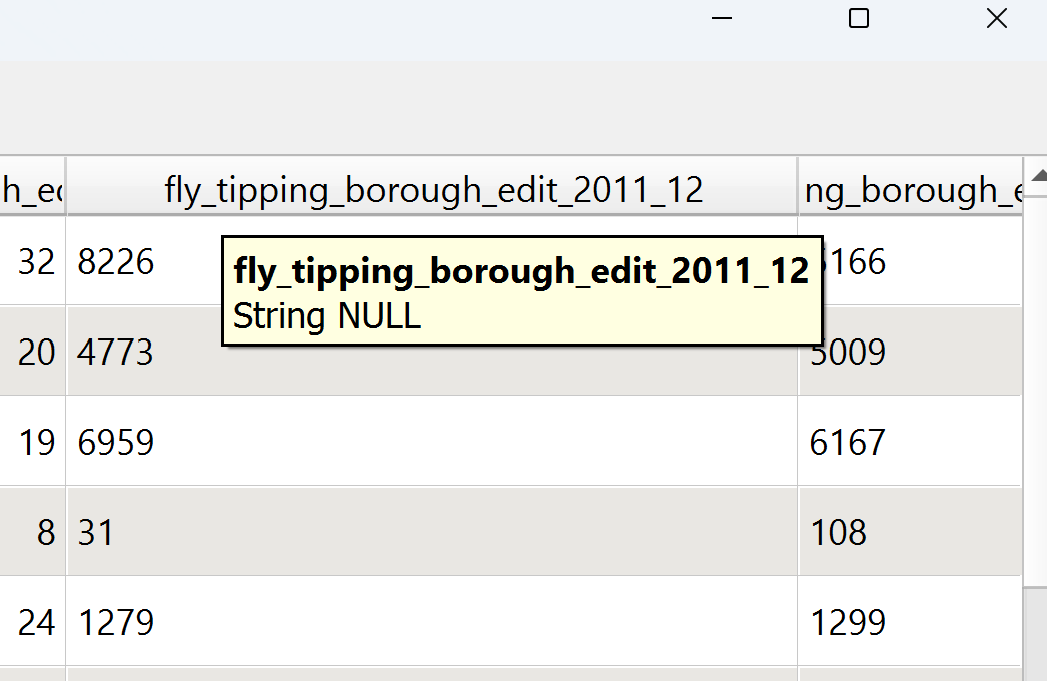
Alternatively we can covert the column type to numeric and selected graduated (for numeric columns). We will convert between text and numeric columns in future weeks.
- Save your QGIS project
You should have produced something like this:
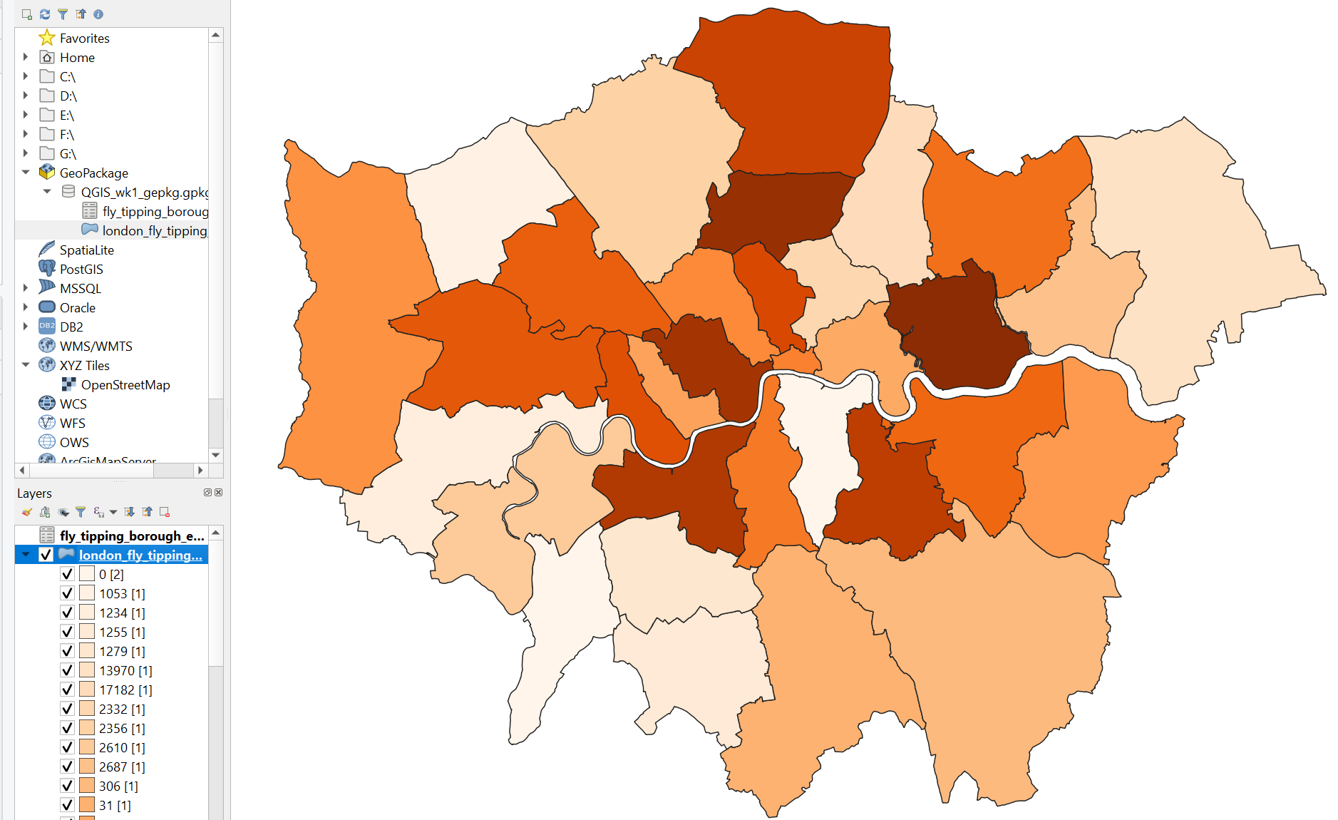
This a very basic map and we’ve just used raw counts to show how to join and map data. You should (almost) never do this, as counts can be misleading. This is because the counts are collected over areas of unequal size. It’s best to divide the values by some sort of denominator (e.g. area of borough, population) to normalise the data giving something like occurrence of flytipping per km2 enabling comparison between the boroughs. We cover this in more detail before reading week.
We haven’t talked about the Coordinate Reference System (CRS) (or Spatial Reference System (SRS)) of our map document
A coordinate reference system is a series of parameters that define the coordinate system. Within GIS we use geographic or projected coordinate systems. The former uses a three-dimensional spherical surface to define locations of Earth, whereas the latter is defined on a flat, two-dimensional surface giving it constant lengths, angles and areas. We cover this in much more detail in subsequent weeks.
QGIS defaults to the Coordinate Reference System (CRS) WGS 84, or known by its European Petroleum Survey Group (EPSG) code 4326. However, when you add your first layer it will default the CRS of the layer. We’ll go into the background of EPSG next time.
You can change the CRS by going Project > Properties and selecting CRS in the left hand pane.
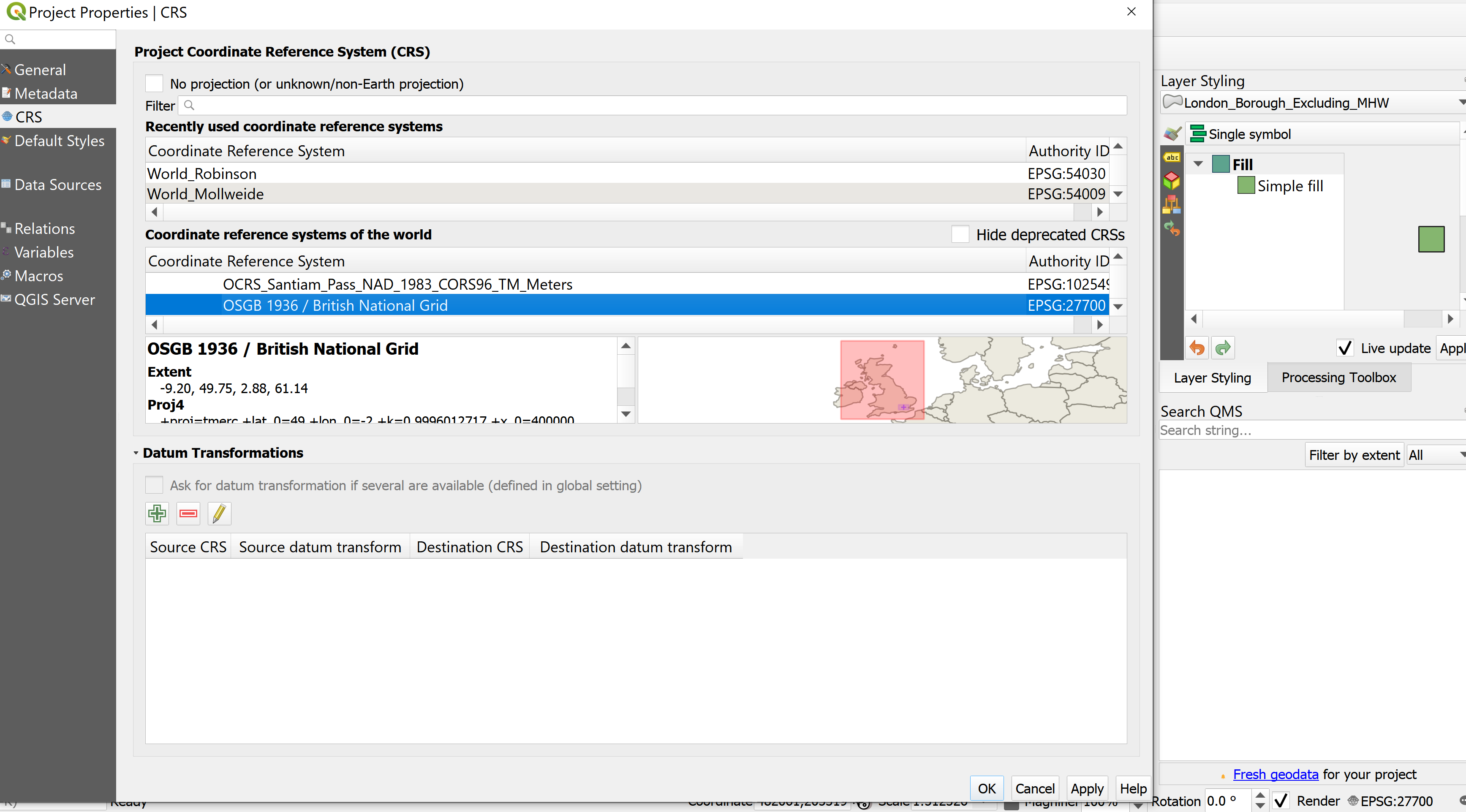
You can also access the project CRS by just clicking on the EPSG code in the bottom right of your QGIS window, in the screenshot above click EPSG:27700.
Note As we are going to open the same files in difference GIS systems it is important to close the software before moving on. If you don’t then files can be locked and unreadable as they are still considered to be in use.