Chapter 10 Advanced R, MAUP and more regression

10.1 Learning outcomes

Describe, explain and visualise the MAUP problem
Design and use loops and functions
Execute linear, Ridge and LASSO regression to predict values (e.g. future or missing)
Critically evaluate different regression approaches

10.2 Homework

Outside of our schedulded sessions you should be doing around 12 hours of extra study per week. Feel free to follow your own GIS interests, but good places to start include the following:

Assignment

From weeks 10 until the assignment deadline, undertake your analysis, then write up your discussion and conclusion (that includes recommendations).

Before submission

Check that your assignment follows the standard model of scientific investigation. You may need to update your introduction and literature review based on the analysis you undertook to ensure a seamless narrative throughout.

Reading This week:

For advanced R coding Chapter 5 “Control flow” from Advacned R by Hadley Wickham.
For more advanced R inclduing functions Chapter 10 “Scripts, algorithms and functions” from Geocomputation with R by Lovelace, Nowosad and Muenchow (2020).
For Ridge and LASSO regression Chapter 4 “Linear models III: shrinkage, multivariate response, and big data” from Predictive Modeling by Portugués (2020).

Remember this is just a starting point, explore the reading list, practical and lecture for more ideas.

10.3 Recommended listening 🎧

Some of these practicals are long, take regular breaks and have a listen to some of our fav tunes each week.

Andy

Adam6 letters: LSB, DRS. Oh yes!

10.4 Introduction

The Modifiable Areal Unit Problem (MAUP) represents the related effects of scale and aggregation on all geographic data and analysis. It was first deomstrated by the geographer Stan Openshaw in 1984 who showed that as you aggregated results to diffrent spatial units the reults could be manipulated to show different outcomes. Throughout this practical book we’ve considered London boroughs, but would any of the results change if we considered the data at ward level? Are we hiding any trends because we have just used the borough data that summed all of the wards within the borough? It’s important to consider what is the most appropriate spatial unit for your analysis and provide appropriate reasoning. Even this is pretty straightforward (e.g. the data was only provided at the borough level) you must contextualise this and describe any potential limitations of it. In this practical i will firstly demonstrate the MAUP in action using some more advanced R code. Then we will have a look at some techniques to model and validate data.

Here we will be using London brough and ward data from practical 1. As we’re getting better with R, we will try to automate almost everthing — meaning that if you gave this code to someone else they could just run it without any data files and generate the same result. The only thing we won’t automate later on is loading an excel file… i did find a function online that would let us read it from the interweb but it was more hassle than it was worth. I don’t know why the data isn’t just also distributed as a .csv.

10.5 MAUP

10.5.1 Get the data

Download and unzip the London statistical gis boundaries.

# make a temp file to store the .zip in

download.file("https://data.london.gov.uk/download/statistical-gis-boundary-files-london/9ba8c833-6370-4b11-abdc-314aa020d5e0/statistical-gis-boundaries-london.zip", 
              destfile="prac10_data/statistical-gis-boundaries-london.zip")

library(tidyverse)
library(fs)
listfiles<-dir_info(here::here("prac10_data")) %>%
  dplyr::filter(str_detect(path, "statistical-gis-boundaries-london.zip")) %>%
  dplyr::select(path)%>%
  pull()%>%
  #print out the .gz file
  print()%>%
  as.character()%>%
  utils::unzip(exdir=here::here("prac10_data"))

## C:/Users/Andy/OneDrive - University College London/Teaching/CASA0005/2020_2021/CASA0005repo/prac10_data/statistical-gis-boundaries-london.zip

Using a recent update we could also change this a bit with the pins() package that downloads and caches the url and automatically checks for file changes, only re-downloading if needed!

library(pins)
pinexample<-pin("https://data.london.gov.uk/download/statistical-gis-boundary-files-london/9ba8c833-6370-4b11-abdc-314aa020d5e0/statistical-gis-boundaries-london.zip")

pins() also lets you share data easily, have a look the RStudio pins blog post for more information.

Take the downloaded data and filter it based on the filename that contains: Borough OR Ward_ AND .shp using grepl()

boroughsandwards<-dir_info(here::here("prac9_data", 
                                 "statistical-gis-boundaries-london", 
                                 "ESRI"))%>%
  #$ means exact match
  dplyr::filter(str_detect(path, 
                        "London_Ward_CityMerged.shp$|London_Borough_Excluding_MHW.shp$"))%>%
  dplyr::select(path)%>%
  pull()

Now read in both of the files using map() that applies a function (here st_read() from the sf package) to a list. map() comes from the purrr package which extends R’s functional programming ability.

library(sf)
boroughsandwardssf<-map(boroughsandwards, st_read)

## Reading layer `London_Borough_Excluding_MHW' from data source `C:\Users\Andy\OneDrive - University College London\Teaching\CASA0005\2020_2021\CASA0005repo\prac9_data\statistical-gis-boundaries-london\ESRI\London_Borough_Excluding_MHW.shp' using driver `ESRI Shapefile'
## Simple feature collection with 33 features and 7 fields
## Geometry type: MULTIPOLYGON
## Dimension:     XY
## Bounding box:  xmin: 503568.2 ymin: 155850.8 xmax: 561957.5 ymax: 200933.9
## Projected CRS: OSGB 1936 / British National Grid
## Reading layer `London_Ward_CityMerged' from data source `C:\Users\Andy\OneDrive - University College London\Teaching\CASA0005\2020_2021\CASA0005repo\prac9_data\statistical-gis-boundaries-london\ESRI\London_Ward_CityMerged.shp' using driver `ESRI Shapefile'
## Simple feature collection with 625 features and 7 fields
## Geometry type: POLYGON
## Dimension:     XY
## Bounding box:  xmin: 503568.2 ymin: 155850.8 xmax: 561957.5 ymax: 200933.9
## Projected CRS: OSGB 1936 / British National Grid

To map or access each individual shapefile it’s just…

library(tmap)
tmap_mode("plot")
qtm(boroughsandwardssf[[2]])

# or change to 1

Get the data for Airbnb

Airbnb <- read_csv("http://data.insideairbnb.com/united-kingdom/england/london/2019-07-10/visualisations/listings.csv")

And for OSM we’ll download it from geofabrik, you can also use the OSM Application Programming Interface (API) but there is a limit on the number of points downloadable per call so you’d have to do something a bit more complicated to get the whole of London…however, I have provided an example of the api call.

library(memisc)
download.file("http://download.geofabrik.de/europe/great-britain/england/greater-london-latest-free.shp.zip",
              mode='wb', 
              destfile="prac10_data/geofabrik.zip")

listfiles<-dir_info(here::here("prac10_data")) %>%
  dplyr::filter(str_detect(path, "geofabrik.zip")) %>%
  dplyr::select(path)%>%
  pull()%>%
  #print out the .gz file
  print()%>%
  as.character()%>%
  utils::unzip(exdir=here::here("prac10_data", "geofabrik"))

Example of using the API….

library(osmar)
src <- osmsource_api(url = "https://api.openstreetmap.org/api/0.6/")
# 1000 refers to distance from centre point
bb <- center_bbox(-0.112510,51.507627, 1000, 1000)
LDN <- get_osm(bb, source = src)
plot(LDN)
# extract just highwways
ways <- find(LDN, way(tags(k == "highway")))
hway <- find_down(LDN, way(ways))
hway <- subset(LDN, ids = hway)

10.5.2 Project the data

Next up we need to project our .shp data …we could project our data individually using:

st_transform(boroughsandwardssf[[1]], 27700)
st_transform(boroughsandwardssf[[2]], 27700)

or use map() again…

boroughsandwardssf<- map(boroughsandwardssf, crs=27700, st_transform)

# change the airbnb data to spatial 
Airbnb <- Airbnb %>%
  st_as_sf(., coords = c("longitude", "latitude"), 
                   crs = 4326)%>%
  # project it too - remember that 27700 is
  # British National Grid
  st_transform(., 27700)

10.5.3 Functions

Now remember our function we made for joining our Airbnb data (or Hotels) to the London boroughs layer… let’s make the function again…

Joinfun <- function(data1, data2){

output<- data1%>%
  st_join(data2,.)%>%
  add_count(GSS_CODE, name="airbnbs") 
  return(output)
}

10.5.4 Loops

Ok, but we want to get a count of Airbnb points per London ward and Borough…how can we do that?…well manually of course…like this…

Airbnbborough <- Joinfun(Airbnb, boroughsandwardssf[[1]])
Airbnbward <- Joinfun(Airbnb, boroughsandwardssf[[2]])

But we can also automate this using a loop (either a while or for loop). I’ve used a while loop here as when i did my MSc you weren’t able to put a for loop inside a for loop. I beleive that has now changed but because of that one day i had to spend changing everything i always default to using a while loop.

Tell us what a loop is already?

A loop let’s you go over something adding 1 (or any value) each time…for example let’s look a basic loop. You need to run everything in the loop at once from the while to the }. If you make just a normal Rscript you can set breakpoints — the code will the stop each time it hits the breakpoint within the loop. You can’t do this at the moment with RMarkdown code chunks, i normally develop the loop outside of it looping then put it all together.

# set up a variable  
basicloop <- 1
# so while our variable is less than 
#6 run the following code within the {}
while (basicloop < 6) {
  #print the varaible (starts at 1)
  print(basicloop)
  # then add 1 to the variable
  basicloop = basicloop+1
  # go back to the start of the loop
  #and if it is still <6 run again
}

## [1] 1
## [1] 2
## [1] 3
## [1] 4
## [1] 5

That loop outputs the values of 1-5, as we started with a value of 1, then added 1 to make 2. It remained below 6 so the code ran again printing the 2 then added 1 again to make 3 and so on. As we specified less than 6 it stopped there..

We can also save these results to diffrent variables but we need to make a list (or dataframe/ whatever you need) to start with to save them in

# here is my empty list
emptylist <- list()
  
basicloop <- 1

while (basicloop < 6) {
  print(basicloop)
  emptylist[[basicloop]] <- basicloop
  basicloop <- basicloop+1
}

## [1] 1
## [1] 2
## [1] 3
## [1] 4
## [1] 5

Here we are using the variable basicloop to index our emptylist.. so everytime we add 1 it changes the index value….have a look what i mean…

emptylist

## [[1]]
## [1] 1
## 
## [[2]]
## [1] 2
## 
## [[3]]
## [1] 3
## 
## [[4]]
## [1] 4
## 
## [[5]]
## [1] 5

emptylist[[1]]

## [1] 1

emptylist[[2]]

## [1] 2

Right, so how are we going to apply this to our data. We have two .shp files (boroughs and wards) in a list that we want to apply our function to..

Firstly let’s set up the length to stop at, make an empty list and a starting point. As our data is in a list we just want the length of that (as a number)..

# get the length - add 1 as we are using less than
boroughlen<-length(boroughsandwardssf)+1
# empty list
hold<-list()
# here is our starting point variable
i<-1

Now here is the loop..

# while i is less than boroughlength 
# max of boroughlength is 3
while (i < boroughlen){
  # put the output in our varible
  # use the function for boroughs and then wards
  hold[[i]] <- Joinfun(Airbnb, boroughsandwardssf[[i]])
  # add one to the index
  i<-i+1
}

# make a quick thematic map to have a look
justairbnbborough<-hold[[1]]%>%
  dplyr::select(GSS_CODE, airbnbs)%>%
  st_drop_geometry()%>%
  distinct(GSS_CODE, airbnbs)%>%
  left_join(boroughsandwardssf[[1]], .,
                        by = c("GSS_CODE" = "GSS_CODE"))

justairbnward<-hold[[2]]%>%
  dplyr::select(GSS_CODE, airbnbs)%>%
  st_drop_geometry()%>%
  distinct(GSS_CODE, airbnbs)%>%
  left_join(boroughsandwardssf[[2]], .,
                        by = c("GSS_CODE" = "GSS_CODE"))

qtm(justairbnbborough, fill = "airbnbs")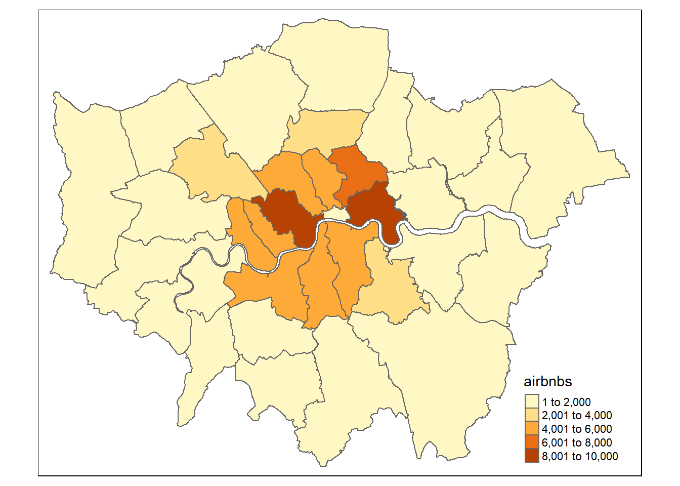

qtm(justairbnward, fill = "airbnbs")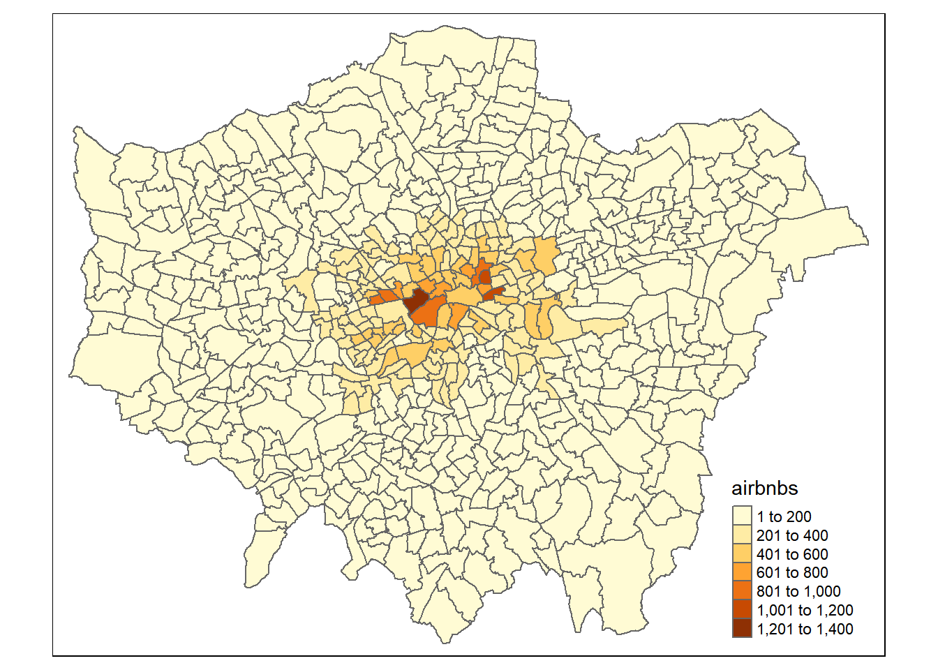

When should i use a loop?

Well that’s a hard question…generally loops used to be considered inefficient in R, but i’m yet to come across a method that will let you increment one varibale whilst keeping another consistent …by this i mean like what we did in our loop. We changed what spatial data was joined with the Airbnb data — the Airbnb data remained the same. There are a few other functions like mapply(), sapply() and tapply() that work in the same format as lapply() but to my knowledge they still will increment all of the variables at the same time.

In terms of code clarity i’m going to refer to section 21.5 on iteration in Wickham $ Grolemund (2017)…

“Some people will tell you to avoid for loops because they are slow. They’re wrong! (Well at least they’re rather out of date, as for loops haven’t been slow for many years). The chief benefits of using ‘other functions’ is not speed, but clarity: they make your code easier to write and to read.”

That said, within this course you are not marked on how ‘good’ or ‘efficient’ your code is. Sure, i want you to write great code, but if you are writing code for your assigment or any future project really, my advice is the same. Get something that works and addresses the mark scheme (read the mark scheme!) and then if you have time, improve it later on. There is also a section later on about writing advanced code in the assignment.

10.5.5 Advanced mapping (again)

Right, so we can sort of see the difference between the spatial levels (boroughs and wards) but let’s take a closer look within Westminster… here is the ‘preamble’ for the leaflet map …basically all the stuff we need to set it up…

library(classInt)
library(leaflet)
library(leafpop)

# extract only westminster from boroughs

Borough <- hold[[1]] %>%
  filter(NAME=="Westminster")%>%
  # we need to set the projection to WGS84
  # to use with leaflet
  st_transform(., crs=4326)%>%
  #at the moment each airbnb is a row for the borough
  #we just one one row that has number of airbnbs
  group_by(., GSS_CODE, NAME)%>%
  summarise(airbnbs = unique(airbnbs))
  
wardsatborough <- hold[[2]] %>%
  filter(BOROUGH=="Westminster")%>%
  # we need to set the projection to WGS84
  # to use with leaflet
  st_transform(., crs=4326)%>%
  #at the moment each airbnb is a row for the wards
  #we just one one row that has number of airbnbs
  group_by(., GSS_CODE, NAME)%>%
  summarise(airbnbs = unique(airbnbs))

# set our breaks for the map
breaks1<-classIntervals(hold[[1]]$airbnbs, 
                        n=5, 
                        style = "quantile")
breaks2<-classIntervals(wardsatborough$airbnbs, 
                        n=5, 
                        style = "quantile")

# use the breaks to set our colour palettes
pal <- colorBin(palette = "YlOrRd", 
                domain=hold[[1]]$airbnbs, 
                bins=breaks1$brks)
pal2 <- colorBin(palette = "YlOrRd", 
                 domain=wardsatborough$airbnbs, 
                 bins=breaks2$brks)

# we want a popup of information too
# here we make a new varaible with no 
#spatial info (remove geometry)

wardinfo <-wardsatborough %>%
  st_drop_geometry()%>%
  dplyr::rename(Ward = NAME,
         Airbnbs = airbnbs)%>%
  dplyr::select(Ward, Airbnbs)%>%
  popupTable()

boroughinfo <-wardsatborough %>%
  st_drop_geometry()%>%
  dplyr::rename(Borough = NAME,
         Airbnbs = airbnbs)%>%
  dplyr::select(Borough, Airbnbs)%>%
  popupTable()

Now let’s map it using what we just specified… i’ve added a few more features than were in the Map making practical

  wardandboroughs<- leaflet() %>%
    # add basemap options
    addProviderTiles(providers$Stamen.TonerLite, group = "Toner Lite") %>%
    addTiles(group = "OSM") %>%
  
    #add our Borough polygons, linking to the tables we just made
    addPolygons(data=Borough,
                color="white", 
                weight = 2,
                opacity = 1,
                dashArray = "3",
                fillOpacity = 0.7,
                popup = boroughinfo,
                fillColor = ~pal(Borough$airbnbs),
                group = "Borough")%>%
    
    #add our ward polygons, linking to the tables we just made
    addPolygons(data=wardsatborough,
                color="white", 
                weight = 2,
                opacity = 1,
                dashArray = "3",
                fillOpacity = 0.7,
                popup = wardinfo,
                fillColor = ~pal2(wardsatborough$airbnbs),
                group = "Wards")%>%
  
    # add a legend for wards
    addLegend(pal = pal2, 
              values = wardsatborough$airbnbs,
              group=c("Wards"), 
              position ="bottomleft",
              title ="Accom count")%>%
     
    # add a legend for boroughs
    addLegend(pal = pal, 
              values = Borough,
              group=c("Borough"), 
              title ="Accom count",
              position ="bottomleft")%>%
  
  # specify layers control
  addLayersControl(
    baseGroups = c("Toner Lite", "OSM"),
    overlayGroups = c("Borough", "Wards"),
    options = layersControlOptions(collapsed = FALSE))%>%
    hideGroup(c("Borough"))

# show us the map
wardandboroughs

Have a look around the map…Westminster borough uses a scale considering all other London borough values, whilst the ward scale is specific to Westminster. Use the following code to explore the values…

# range of Airbnbs per ward in Westminster

Range<-wardsatborough %>%
  summarise(Max = max(airbnbs),
            Min = min (airbnbs))

10.6 Regression relationships

Warning The data used within this practical is purely for demonstration purposes!

10.6.1 Preprocessing

In this part of the practical we’re going to try and model the relationship between the Airbnb counts at ward level and other variables. Our mini investagion here would be to see if it’s possible to produce a statisitcally valid and rigorous model for predicting Airbnb values at the ward level. This type of analysis might be useful if you had missing or limited data at one spatial level (e.g. wards) but had a more complete dataset at a larger spatial scale (e.g. boroughs). Essentially, we’re trying to use the data at the borough level to give us an estiamte of the data at the ward level. Obviously this isn’t an issue for us here but if you ever use survey data or any kind of count data (e.g. health) if may well be limited to specific areas…

This section will also show you how to make/ use different regression models in R. Regression aims to find a mathematical equation to predict a value (in this case Airbnb at ward level) from one (or more) predictor variables (e.g. borough data). So we’ll use values of X (borough data) to predict values of Y (ward data)…

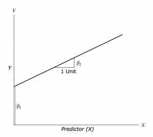
This can be represented with the equation:

\[Y = \beta_{1} + \beta_{2} X + \epsilon\] Where $\beta_{1}$ is the intercept (expected value of Y when X=0, also called bias in machine learning), $\beta_{2}$ is the slope of the line and $\epsilon$ is the error term, the part that the model is unable to explain (and variables are not included)…Here we would call the intercept and slop coefficients.

To start with we’re going to crop our wards data to our boroughs data. In the borough data you can see the river Thames which isn’t in the wards data. I don’t think this is technically required, but it’s good practice to make sure you datasets align and if they don’t to do something about it…

library(tmaptools)

cropped <- justairbnbborough %>%
  crop_shape(justairbnward,., polygon = TRUE)

# something like this would just extract the 
# values within the shape, but not clip like a cookie cutter
# we want to use the borough layer to cut out the river from 
# the wards layer
###test <- hold[[2]][hold[[1]],]

# check it worked, you should be 
#able to see the river

plot(st_geometry(cropped))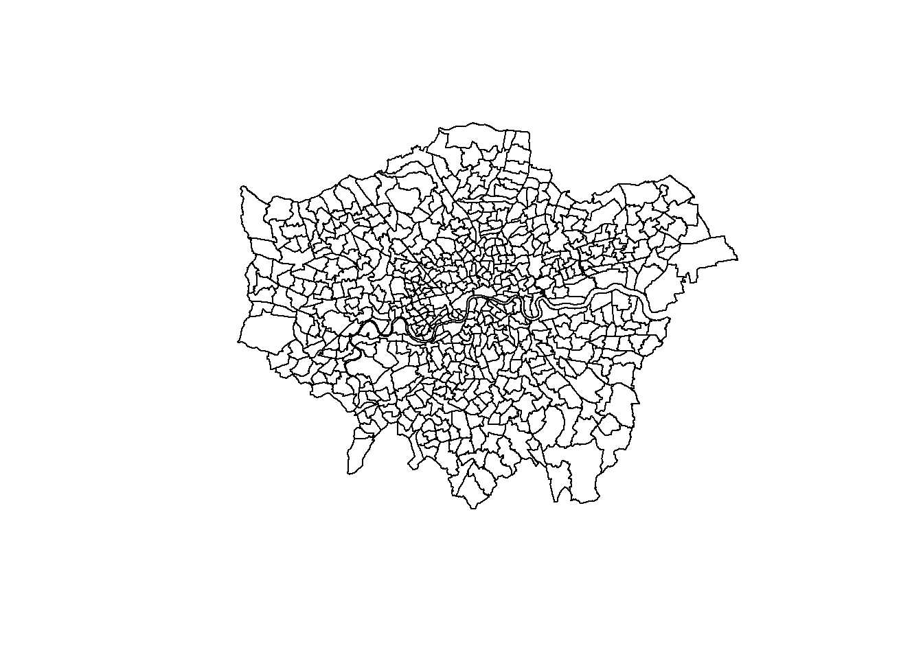

Now we need to join our wards data and borough data togther to give us a borough value for each ward within…

# join wards and boroughs

joined <- justairbnbborough %>%
  st_join(., justairbnward, join=st_contains)%>%
  rename(., Boroughcount = airbnbs.x, 
         Wardcount = airbnbs.y)

10.6.2 Scatter plot

To start with let’s just visualise the relationship between the borough an ward count using a scatter plot. If you have multiple predictor variables (explied later on) a plot will be drawn for each of them…

p <- ggplot(joined, aes(Boroughcount, Wardcount))+
  geom_point()+
  xlab("Borough count")+
  ylab("Ward count")

The scatter plot shows some kind of linear relationship. The point variation around borough count is beacuse for each borough the wards will have a range of values…like we saw in the interactive map…Westminster borough had a value of 9410 and the wards ranged from 159 to 1215

10.6.3 Outliers

Generally any point that is outside 1.5* the interquartile-range (or IQR) is considered an outlier (a data point that differs significantly from all others) and you could use something like the methods here to remove and replace them…the IQR is the distance between the 25th and 75th percentile..

par(mfrow=c(1, 2))  # divide graph area in 2 columns

boxplot(joined$Boroughcount, main="Boroughs")
boxplot(joined$Wardcount, main="Wards")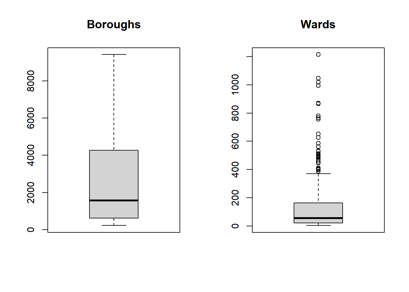

Warning The data used within this practical is purely for demonstration purposes! These box plots indicate that our data is not normally distributed so you might want to refer to the assumptions in last week’s practical if you were to do this propperly.

10.6.4 Correlation

Correlation let’s use see the level of linear dependence between two varaibles between -1 and 1. High values (towards 1) mean that for every x instance there is an increase in y. Low values (towards -1) mean the opposite.

library(corrr)

Correlation <- joined %>%
  st_drop_geometry()%>%
  dplyr::select(Boroughcount,
                Wardcount)%>%
    correlate() %>%
  print()

## # A tibble: 2 x 3
##   term         Boroughcount Wardcount
##   <chr>               <dbl>     <dbl>
## 1 Boroughcount       NA         0.789
## 2 Wardcount           0.789    NA

Looks, like we’ve got a strong relationship.

10.6.5 Linear model

Now let’s use a linear model to establish a relationship between predictor and response with the function lm(). Here we are calling the lm()(then stating the Formula, then the data)

library(broom)
linearMod <- lm(Wardcount ~ 
                  Boroughcount, 
                data=joined)

tidy(linearMod)

## # A tibble: 2 x 5
##   term         estimate std.error statistic   p.value
##   <chr>           <dbl>     <dbl>     <dbl>     <dbl>
## 1 (Intercept)  -10.9      6.20        -1.76 7.97e-  2
## 2 Boroughcount   0.0550   0.00182     30.2  2.68e-119

So from this output we have the coefficients of intercept and Boroughcount, going back to our formula from earlier this would mean…

\[Wardcount = -3.8188 + 0.0541*Boroughcount\]

10.6.6 Linear model outputs

Coefficient Estimates

Our intercept, the expected value of Y when X=0 is -3.8 and slope is 0.054.

Standard error

The coefficient standard error represents the average amount that coeffieint estimates vary from the average of our response. It basically shows the expected range if we were to model again and again. So here, for a 1% increase in the number of Airbnbs per ward by 0.05, but this might vary by 0.001. Ideally the standard error is lower than the size of the coeffeicient (0.001 is lower the 0.05)

p-value

A linear model is only statistically significant when both p-values are <0.05 within the summary call. There are two values as one if for the coefficient (is the specific coefficient significant) and the other is for the model (is the model significant). Here as they both are, this would allow us to accept the alternative hypothesis that the coefficients are not equal to 0 (and therefore there is a relationship between the independent and dependent variabile).

R-squared

R squared represents the proportion of variance of the dependent variable that is explained by the independent. It is different from correlation as that is the strength of the relationship!!! R squared is often referred to as ‘goodness-of-fit.’ Here 61% of the variance in Airbnb ward count can be explained by the varaition in Airbnb borough count.

But there are a few issues with R squared — every time you add a predictor to the model R squared will increase and if there are too many predictors it will model random noise

Adjusted R squared

Adjusted R squared consideres the number of variables within the model, increasing only if the new term assits by more than just chance.

Coefficient t shows how many standard deviations the coefficient estaimte is away from 0 — the further away means the more likely we can reject the null hypothesis. It is calcaulted by dividing the value of the coeffeicient by the standard error

Residual error

Residual standard error is a measure of the quality of fit of the linear regression line. It is an average of the error that the points differ out from the line.

F-statistcs, basically, the futher from 1 the better it is.

See this guide for more information on the outputs

Remember the formula produced from the regression equation, well we can also extract this automatically …to make that original formula in RMarkdown I used this (not within a code chunk)….

$$Wardcount = -3.8188 + 0.0541*Boroughcount$$

But we can also extract it directly using a new package from GitHub…

# load remotes so we can get the new package
library(remotes)

# get the new package equatiomatic()
remotes::install_github("datalorax/equatiomatic")

# load it
library(equatiomatic)
# extract the info to make the equation
extract_eq(linearMod)

\[ \operatorname{Wardcount} = \alpha + \beta_{1}(\operatorname{Boroughcount}) + \epsilon \]

Play around with line length and use the actual coefficient names

extract_eq(linearMod, use_coefs = TRUE, wrap=TRUE, terms_per_line = 2)

\[ \begin{aligned} \operatorname{\widehat{Wardcount}} &= -10.89 + 0.06(\operatorname{Boroughcount}) \end{aligned} \]

This would produce the following in RMarkdown….

\[ \begin{aligned} \text{Wardcount} &= -3.82 + 0.05(\text{Boroughcount})\ + \\ &\quad \epsilon \end{aligned} \]

Have a look here for more information on using equatiomatic().

10.6.7 Validation

We’ve made a regression model using all of our data but there is now no way to test its validity…what if we take 20% as a test sample and use the remaining 80% to train it…

joinedID <- joined %>% 
  st_drop_geometry()%>%
  mutate(Wardcount = replace_na(Wardcount, 0))%>%
  mutate(id = row_number())
# Create training 80% index
train <- joinedID %>% 
  sample_frac(.70)
# Create test set
test  <- anti_join(joinedID, 
                   train, 
                   by = 'id')

Now let’s build the model…

# build the model
lmMod <- lm(Wardcount ~ Boroughcount, 
            data=train)  
# use the model to make some predicitons with our test data

library(caret)
predictions <- lmMod %>% 
  predict(test)

# get R2, RMSE and MAE

stats<-data.frame(R2 = R2(predictions, test$Wardcount),
            RMSE = RMSE(predictions, test$Wardcount),
            MAE = MAE(predictions, test$Wardcount))

t

## Warning in print.summary.sarlm(x): install the spatialreg package

## 
## Call:
## lagsarlm(formula = average_gcse_capped_point_scores_2014 ~ unauthorised_absence_in_all_schools_percent_2013 + 
##     log(median_house_price_2014), data = LonWardProfiles, listw = nb2listw(LWard_nb, 
##     style = "C"), method = "eigen")
## 
## Residuals:

## Warning in residuals.sarlm(x): install the spatialreg package

##       Min        1Q    Median        3Q       Max 
## -73.47436 -10.22693  -0.21223   8.94538  50.92267 
## 
## Type: lag 
## Coefficients: (asymptotic standard errors) 
##                                                  Estimate Std. Error  z value
## (Intercept)                                      202.3427    20.0987  10.0675
## unauthorised_absence_in_all_schools_percent_2013 -36.1756     1.9136 -18.9045
## log(median_house_price_2014)                      12.5878     1.5327   8.2127
##                                                   Pr(>|z|)
## (Intercept)                                      < 2.2e-16
## unauthorised_absence_in_all_schools_percent_2013 < 2.2e-16
## log(median_house_price_2014)                      2.22e-16
## 
## Rho: 0.0051568, LR test value: 0.46178, p-value: 0.49679
## Asymptotic standard error: 0.0075929
##     z-value: 0.67916, p-value: 0.49704
## Wald statistic: 0.46126, p-value: 0.49704

## Warning in logLik.sarlm(x): install the spatialreg package

## Warning in residuals.sarlm(object): install the spatialreg package

## 
## Log likelihood: -2603.509 for lag model
## ML residual variance (sigma squared): 239.86, (sigma: 15.487)
## Number of observations: 626 
## Number of parameters estimated: 5

## Warning in logLik.sarlm(object): install the spatialreg package

## Warning in logLik.sarlm(object): install the spatialreg package

## AIC: 5217, (AIC for lm: 5215.5)
## LM test for residual autocorrelation
## test value: 131.82, p-value: < 2.22e-16

#for some reason this will show in RStudio
#but not the bookdown (this practical) output.

We can use the R2, Root Mean Square Error and Mean Absolute Error.

$R^2$ is the variation of y explained by x
Mean Absolute Error measures the average magnitude of the errors (distance of points from the regression line) using:

\[MAE = {\frac{1}{n}\Sigma_{i=1}^{n}{\Big({d_i -f_i\Big)}}}\]

Root Mean Square Error (RMSE) is the standard deviation of the resuiduals, this means how far away the points are from the regression line…

\[RMSE= \sqrt{\frac{1}{n}\Sigma_{i=1}^{n}{\Big({d_i -f_i}\Big)^2}}\] Where $d_i$ is the actual value, $d_f$ is the predicted value, and $n$ is the number of data points

We could also just run a correlation between the data we left out and the predicted data to assess the accuracy…

actuals_preds <- data.frame(cbind(actuals=test$Wardcount,
                                  predicteds=predictions))


actuals_preds_correlation <- actuals_preds %>%
    correlate() %>%
  print()

## # A tibble: 2 x 3
##   term       actuals predicteds
##   <chr>        <dbl>      <dbl>
## 1 actuals     NA          0.776
## 2 predicteds   0.776     NA

This shows us that we have a strong and significant relationship between our model output and the test data.

We can also use min-max accuracy to see how close the actual and predicted values are…using the equation…

\[MinMaxAccuracy= mean\left( \frac{min(actuals, predicteds}{max(actuals, predicteds)} \right)\]

min_max_accuracy <- mean(apply(actuals_preds, 1, min, na.rm=TRUE) /
                          apply(actuals_preds, 1, max, na.rm=TRUE))  
min_max_accuracy

## [1] 0.5168844

This gives around a 60% accuracy…another alternative is mean absolute percentage deviation which is a statistical measure showing how accurate the prediciton was…through the equation…

\[MAPE= mean\left( \frac{abs(predicteds - actuals}{actuals} \right)\]

mape <- mean(abs((actuals_preds$predicteds -
                    actuals_preds$actuals))/
               actuals_preds$actuals, na.rm=TRUE)  

mape

## [1] Inf

Here we’ve got a very high MAPE — this is most likely because of the range of values of the wards for individual boroughs…

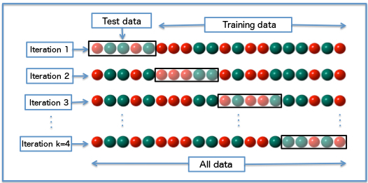
10.6.8 Cross validation

Our validation approach so far was OK, but what if the test data was a different 20% — would it still hold up? We can test this by dividing all our data into blocks and then running the analysis several times, each time selecting a different block to be the test data…this is called cross validation …

To start with we’ll remove the geomtery, set up a data frame and replace any NAs with 0 — this is appropraite here as if there are no Airbnbs within the ward they would be 0.

joined_CV <- joined %>%
  st_drop_geometry()%>%
  mutate(Wardcount = replace_na(Wardcount, 0))

Now let’s change our training data… here i’ve got 5 iterations then the whole lot is repeated 3 times. Search literautre for the right number to use, i think 10 iterations with no repeats is a good place to start.

library(caret)
model<- train(Wardcount ~ Boroughcount, 
              joined_CV,
              method="lm", 
              trControl=trainControl(method="repeatedcv",
                                     number=5,
                                     repeats=3,
                                     # change to true to
                                     # see it iterate
                                     verboseIter=FALSE))

summary(model)

## 
## Call:
## lm(formula = .outcome ~ ., data = dat)
## 
## Residuals:
##     Min      1Q  Median      3Q     Max 
## -347.88  -38.61    0.26   20.97  708.12 
## 
## Coefficients:
##                Estimate Std. Error t value Pr(>|t|)    
## (Intercept)  -10.935710   6.184881  -1.768   0.0776 .  
## Boroughcount   0.055028   0.001816  30.294   <2e-16 ***
## ---
## Signif. codes:  0 '***' 0.001 '**' 0.01 '*' 0.05 '.' 0.1 ' ' 1
## 
## Residual standard error: 100.7 on 554 degrees of freedom
## Multiple R-squared:  0.6236, Adjusted R-squared:  0.6229 
## F-statistic: 917.7 on 1 and 554 DF,  p-value: < 2.2e-16

#print R2, MAE and RMSE
print(model)

## Linear Regression 
## 
## 556 samples
##   1 predictor
## 
## No pre-processing
## Resampling: Cross-Validated (5 fold, repeated 3 times) 
## Summary of sample sizes: 444, 447, 445, 444, 444, 444, ... 
## Resampling results:
## 
##   RMSE      Rsquared   MAE     
##   99.65453  0.6364164  57.45796
## 
## Tuning parameter 'intercept' was held constant at a value of TRUE

Results show that our cross validated model accounts for around 60% of varaince of the number of Airbnbs per ward…compare this to the results from the standard linear regression…

10.7 Advanced regression

10.7.1 More data

We’re going to have a look at Ridge and LASSO regression next…however, they require us to have more than 1 predictor variable, so we’ll load a few in and demonstrate how to use them in normal regression first…

We’ll get our OSM data, project it, extract only hotels, join it with the boroughs, set any NAs to 0, join it with the wards, rename the new ‘freq’ coloumn to Hotel count, remove the geometry and then set any more NAs to 0…

# read in OSM data
OSM <- st_read(here::here("prac10_data", "geofabrik", "gis_osm_pois_a_free_1.shp"))

## Reading layer `gis_osm_pois_a_free_1' from data source `C:\Users\Andy\OneDrive - University College London\Teaching\CASA0005\2020_2021\CASA0005repo\prac10_data\geofabrik\gis_osm_pois_a_free_1.shp' using driver `ESRI Shapefile'
## Simple feature collection with 37108 features and 4 fields
## Geometry type: MULTIPOLYGON
## Dimension:     XY
## Bounding box:  xmin: -0.5108706 ymin: 51.28117 xmax: 0.322123 ymax: 51.68948
## Geodetic CRS:  WGS 84

# project and filter
OSM <- OSM %>%
  st_transform(., 27700) %>%
  filter(fclass == "hotel")

# join hotels with the boroughs

Hotels_borough <- OSM %>%
  Joinfun(., boroughsandwardssf[[1]]) %>%
  # rename hotels
  dplyr::rename(hotels = airbnbs) %>%
  # replae NA with 0
  mutate(hotels = replace_na(hotels, 0))


joined2<-joined %>%
  st_drop_geometry()%>%
  left_join(., 
            Hotels_borough,
            by= c("GSS_CODE.x" = "GSS_CODE"))%>%
  dplyr::select(NAME.y,GSS_CODE.x, Boroughcount, Wardcount, hotels)%>%
  distinct()%>%
  #replace NA in wards with 0
  mutate(Wardcount = replace_na(Wardcount, 0))

10.7.2 Multiple linear regression

Re run the model including Hotel count…you simply use a +

model2<- train(Wardcount ~ Boroughcount+hotels, 
              joined2,
              method="lm", 
              trControl=trainControl(method="repeatedcv",
                                     number=5,
                                     repeats=3,
                                     # change to true to see it 
                                     # iterate
                                     verboseIter=FALSE))

summary(model2)

## 
## Call:
## lm(formula = .outcome ~ ., data = dat)
## 
## Residuals:
##     Min      1Q  Median      3Q     Max 
## -340.04  -38.24    0.51   21.02  715.96 
## 
## Coefficients:
##                Estimate Std. Error t value Pr(>|t|)    
## (Intercept)  -11.485809   6.342871  -1.811   0.0707 .  
## Boroughcount   0.055620   0.002351  23.656   <2e-16 ***
## hotels        -0.033929   0.085485  -0.397   0.6916    
## ---
## Signif. codes:  0 '***' 0.001 '**' 0.01 '*' 0.05 '.' 0.1 ' ' 1
## 
## Residual standard error: 100.8 on 553 degrees of freedom
## Multiple R-squared:  0.6237, Adjusted R-squared:  0.6223 
## F-statistic: 458.2 on 2 and 553 DF,  p-value: < 2.2e-16

The summary here shows that the hotel count predictor is not statistically significant so we should remove it…how about we add some population and house price data….download the excel data from here

library(readxl)
library(janitor)
# read the excel sheet
my_data <- read_excel(here::here("prac10_data","ward-profiles-excel-version.xls"),
                                 sheet=2,
                                 col_names=TRUE) %>%
  # set it as a data frame
  as.data.frame()%>%
  clean_names()%>%
  # extract everything that begins with E
  filter(str_detect(new_code, "^E"))

# is our data num
Datatypelist <- my_data %>% 
  summarise_all(class) %>%
  pivot_longer(everything(), 
               names_to="All_variables", 
               values_to="Variable_class")

# make sure the variables are numeric
my_data <- my_data %>%
  mutate(across(.cols = 4:67, as.numeric))

# merge the new data to the existing data
joined3 <-joined2 %>%
  left_join(.,
            my_data,
            by= c("GSS_CODE.x" = "new_code"))

Now run the model again

model3<- train(Wardcount ~ Boroughcount+population_2015
               +median_house_price_2014,
              joined3,
              method="lm", 
              trControl=trainControl(method="repeatedcv",
                                     number=5,
                                     repeats=3,
                                     verboseIter=FALSE))

summary(model3)

## 
## Call:
## lm(formula = .outcome ~ ., data = dat)
## 
## Residuals:
##     Min      1Q  Median      3Q     Max 
## -351.59  -34.88   -3.98   21.15  704.41 
## 
## Coefficients:
##                           Estimate Std. Error t value Pr(>|t|)    
## (Intercept)              3.664e+01  2.878e+01   1.273   0.2035    
## Boroughcount             5.432e-02  2.623e-03  20.709   <2e-16 ***
## population_2015         -1.700e-04  7.873e-05  -2.159   0.0313 *  
## median_house_price_2014  2.218e-06  3.544e-05   0.063   0.9501    
## ---
## Signif. codes:  0 '***' 0.001 '**' 0.01 '*' 0.05 '.' 0.1 ' ' 1
## 
## Residual standard error: 100.2 on 553 degrees of freedom
## Multiple R-squared:  0.6281, Adjusted R-squared:  0.626 
## F-statistic: 311.3 on 3 and 553 DF,  p-value: < 2.2e-16

Our R squared and adjusted R squared have increased (albeit slightly) and all predictors are statistically significant.

Note that whilst i have selected variables pretty randomly here for demonstration, if you use something like this in practice it’s important to have supported (referenced) reasoning behind your selections.

10.7.3 Ridge regression

Least squares regression tries to minimise how far each point is away from the line…but if you look in this figure…the red dots are the training data and the green dots are the test data. Here normal OLS has been fitted to the training data perfectly…the sum of the squared residuals (squared error distance from the line) is very small, probably 0. But when applied to the test data the sum of the squared residuals is large — it therefore has high variance and would be termed to be overfitting the training data.

Figure 10.1: This is a screenshot from the YouTube video Regularization Part 1: Ridge Regression by StatQuest

Ridge regression probably won’t fit our training data as well, because we introduce a small amount of bias (adding value to the intercept — which is the Y value when X=0, normally making the line of best fit more horizontal) to give us less overall variance (the difference between the point and line value)…So essentially when the values are calculated the formula is trying to get the line of best fit through all the points with each point having minimum distance to the line. This is usually useful in trying to get predicitions from the model.

Ridge regression also tries to minimise the sum of the squared residuals (distance to the line) but then adds $\lambda$ x $slope^2$ — this is the bias changing the line of best fit

Ok so let’s try and look at this with numbers…

The goal here is to minimise the sum of the squared residuals…plus the ridge regression penalty $\lambda * slope^2$…

Firstly let’s assume you have a perfectly fit line — the sum of the least sqaure residuals would be 0 (the line overlaps the points). Assume $\lambda$ is 0.5 and the slope is 1.2, we have 0 (residuals) + 0.5 ($\lambda$) * 1.44 (slope squared) = 0.72

Now we use ridge regression that shifts the line away from the perfect fit (with a bias penalty) that we had in least square regression…this would create residual values as the points no longer perfectly fit the line, assume these add to 0.2, $\lambda$ is 0.5, and the slope is 0.7…so this would give….0.2 (residuals) + 0.5 ($\lambda$) * 0.49 (slope squared) = 0.445.

So if we were trying to minimise the sum of the squared residuals plus the ridge regression penalty the ridge regression wins with a lower value.

The penalty $\lambda * slope^2$ adds a bias (value to the intercept) to reduce the slope of the line as it tries to the minimise the sum of the distance of the points from the line and hopefully the variance between the line and the points…like this — Ridge is the blue line that has become slightly more horizontal…

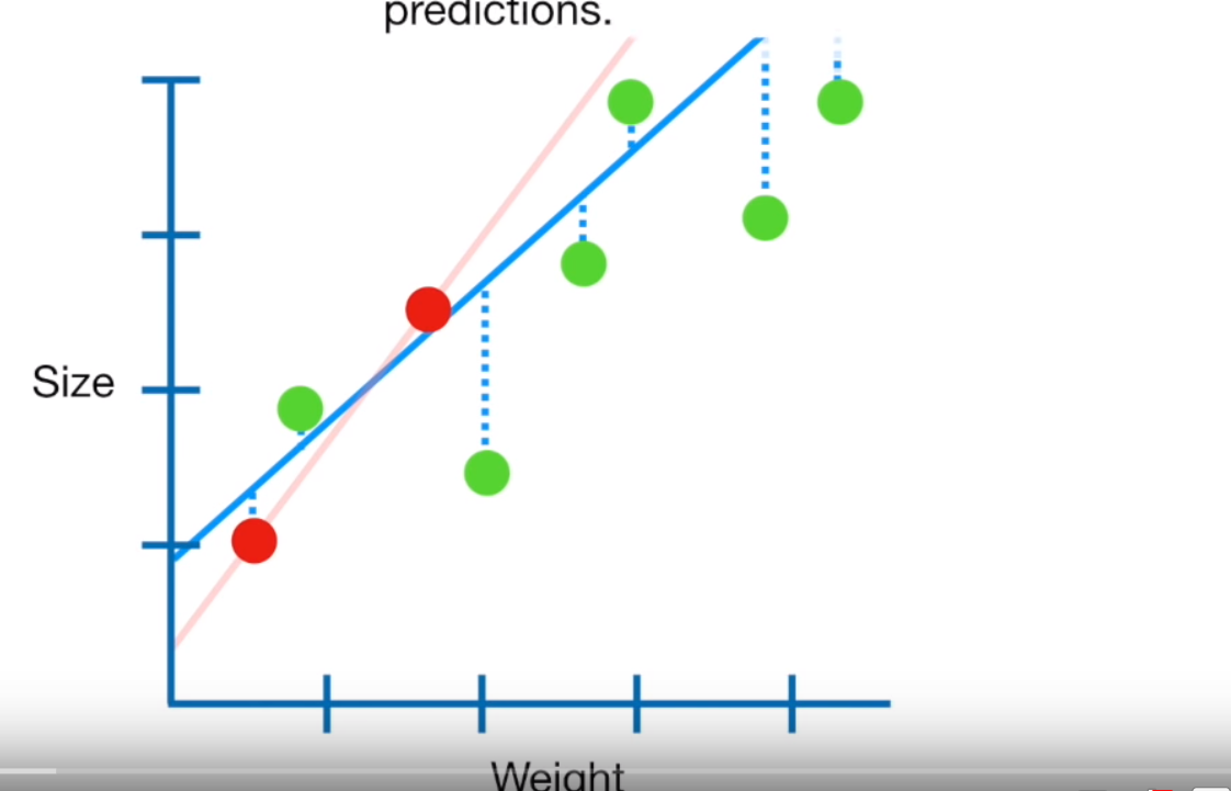
Figure 10.2: This is a screenshot from the YouTube video Regularization Part 1: Ridge Regression by StatQuest

But wait…. how do we calculate $\lambda$, well we try a load of values and use cross validation (10 fold) to get the overall lowest variance from the line to the data points! COOL!!!!

Let’s see an example to show that if $\lambda$ is 0, then we have our box standard linear regression…as the penalty $\lambda * the slope^2$ will be 0, so we will just be minimising the sum of the squared residuals.

library(tidyverse)
library(broom)
library(glmnet)


# sort the data our for ridge regression
y <- joined3$Wardcount %>%
  # set NAs to 0
  replace_na(., 0)

x <- joined3 %>% 
  dplyr::select(Boroughcount, hotels,
                                 population_2015,
                                 median_house_price_2014) %>%
  data.matrix()%>%
  # set NAs to 0
  replace_na(., 0)


# set seed means that if we re run this 
# we will get the same results
set.seed(489)
# this gives us a 50/50 split between
# training and test data
train = sample(1:nrow(x), nrow(x)/2)
test = (-train)
ytest = y[test]
xtest =x[test]

# run normmal regression
normallm <- lm(Wardcount ~ hotels+Boroughcount+population_2015
               +median_house_price_2014,
               data = joined3)
summary(normallm)

## 
## Call:
## lm(formula = Wardcount ~ hotels + Boroughcount + population_2015 + 
##     median_house_price_2014, data = joined3)
## 
## Residuals:
##     Min      1Q  Median      3Q     Max 
## -334.19  -35.85   -2.95   20.95  721.81 
## 
## Coefficients:
##                           Estimate Std. Error t value Pr(>|t|)    
## (Intercept)              3.175e+01  2.935e+01   1.082   0.2798    
## hotels                  -7.851e-02  9.174e-02  -0.856   0.3925    
## Boroughcount             5.506e-02  2.761e-03  19.944   <2e-16 ***
## population_2015         -1.679e-04  7.878e-05  -2.132   0.0335 *  
## median_house_price_2014  1.350e-05  3.782e-05   0.357   0.7213    
## ---
## Signif. codes:  0 '***' 0.001 '**' 0.01 '*' 0.05 '.' 0.1 ' ' 1
## 
## Residual standard error: 100.3 on 552 degrees of freedom
## Multiple R-squared:  0.6286, Adjusted R-squared:  0.6259 
## F-statistic: 233.5 on 4 and 552 DF,  p-value: < 2.2e-16

# make a variable for loads of lambda values
# just for the example here
lambda <- 10^seq(10, -2, length = 100)

#run ridge regression, here we use x to predict y
ridge_mod <- glmnet(x, y, alpha = 0, lambda = lambda)
# x and y are our original data,
#s is the size of the penalty which is 0
# and we want the coefficients out
predict(ridge_mod, x=x,y=y, s = 0, exact = T, type = 'coefficients')

## 5 x 1 sparse Matrix of class "dgCMatrix"
##                                     1
## (Intercept)              3.172445e+01
## Boroughcount             5.505627e-02
## hotels                  -7.854144e-02
## population_2015         -1.678941e-04
## median_house_price_2014  1.353453e-05

The coefficient estaimtes should be the same or very very similar…now let’s try and use ridge regression to improve upon our least squares regression…first let’s show linear regression for comparison using the train data..

normallm2 <- lm(Wardcount ~ hotels+Boroughcount+population_2015
               +median_house_price_2014, 
               data = joined3, 
               subset = train)


s_pred <- predict(normallm2, newdata = joined3[test,])
mean((s_pred-ytest)^2)

## [1] 8068.011

Now we will find the best value for $\lambda$ using cross validation

#find the best lambda from our list via cross-validation
# family = gaussian means linear regression
# type.measure = how cross evaluation will be evaluated 
# mse is mean square error
cv_out <- cv.glmnet(x[train,], 
                    y[train],
                    alpha = 0, 
                    family="gaussian",
                    type.measure = "mse")

Combined, this will fit a linear regression with a ridge regression penatly using 10-fold cross validation to find the best $\lambda$ value that minimises mean square error (average squared distance of the data points to the line). Let’s apply it to the model…

plot(cv_out)

# best value 
opt_lambda <- cv_out$lambda.min

# prediction to the testing data
# s is set to optimal lambda
# you could also use lambda.1se as
# technically they are indistinguishable 
ridge_pred <- predict(ridge_mod, s = opt_lambda, newx = x[test,])

# rsquared
ridge_r <- cor(y[test], ridge_pred)^2
ridge_r

##              1
## [1,] 0.6543214

# mean square error
mean((ridge_pred-ytest)^2)

## [1] 7134.638

You can also doing this in a few less steps with the ridge package

10.7.4 LASSO

Least absolute shrinkage and selection operator (LASSO) performs variable selection and regularisation to increase prediction accuracy of the model…the only difference to ridge is that the regularisation term is an absolute value. So instead of squaring the slope (like i mentioned in Ridge regression), we take the absolute value (of the slope, as opposed the the squared value in Ridge) and as the slope can be 0 it can be removed from the model. As a result LASSO regression can increase $\lambda$ then set irrelevant parameters to 0 (Ridge will just shrink them but not set to 0) — relevant parameters might shrink a little bit in both too. The advantage here is that LASSO can exclude useless variables — so if you have a lot of variables it might be preferable. However, if most variables are useful then Ridge regression would probably work better.

LASSO has an absolute penalty (also known as L1 penalty)
Ridge has a square penalty (also known as L2 penalty)

#find the best lambda from our list via cross-validation
cv_out <- cv.glmnet(x[train,], 
                    y[train], 
                    alpha = 1, 
                    family="gaussian", 
                    type.measure = "mse")

plot(cv_out)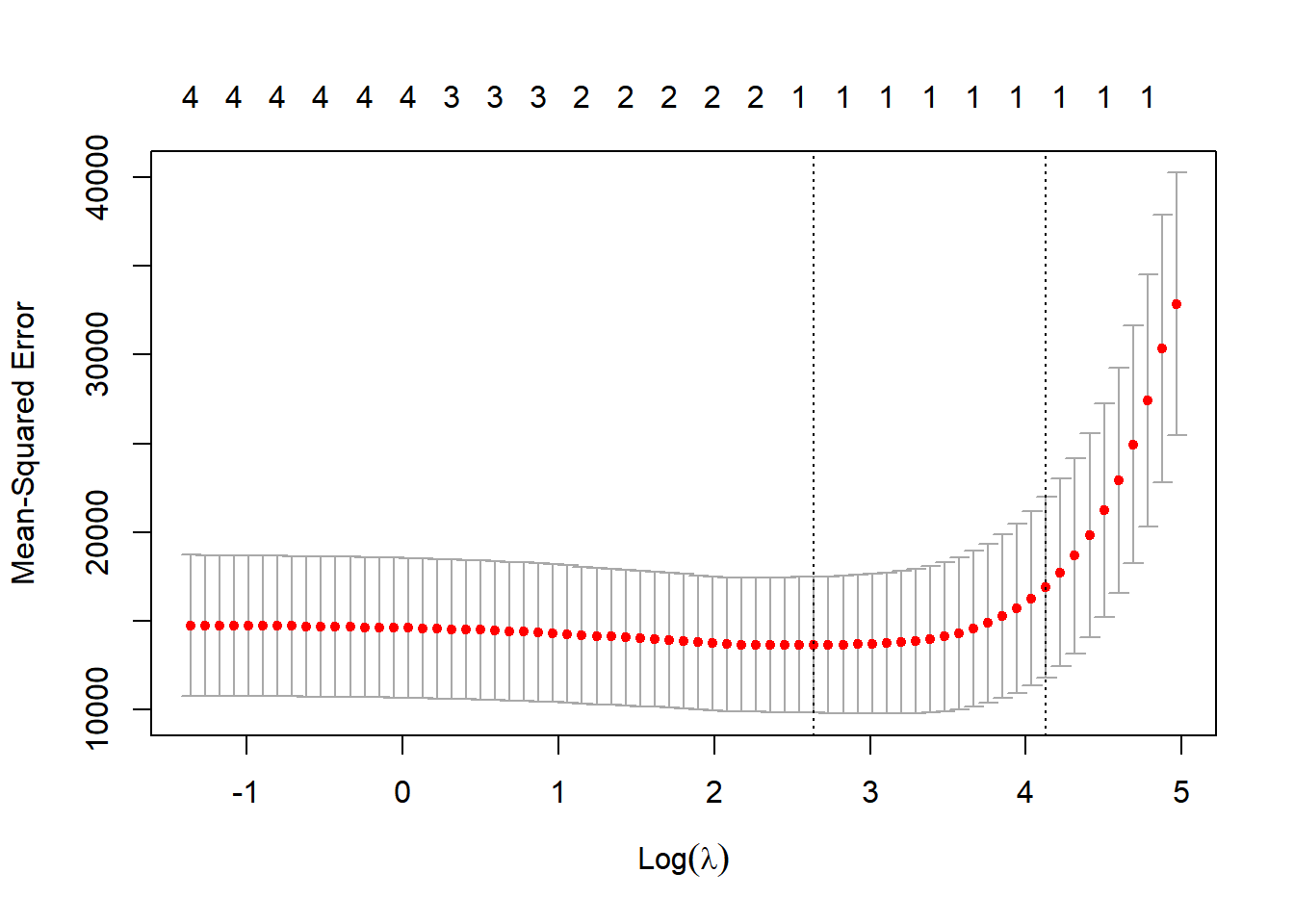

# best value 
opt_lambda <- cv_out$lambda.min

# make the model
lasso_mod <- glmnet(x[train,], y[train], alpha = 1, lambda = opt_lambda)

# make the prediction 
lasso_pred <- predict(lasso_mod, s = opt_lambda, newx = x[test,])

# r sqaured
LASSO_r <- cor(y[test], lasso_pred)^2
LASSO_r

##              1
## [1,] 0.6423348

# mean square error
mean((lasso_pred-ytest)^2)

## [1] 7588.756

10.7.5 Elastic net regression

When you don’t know much about our variables in a model you can use Elastic-Net Regression. It starts with least squares then adds the LASSO and ridge regression penalty, allowing you to use the strengths of both. Both the LASSO penalty and ridge penalty get their own $\lambda$ values, $\lambda_1$ for LASSO, $\lambda_2$ for ridge. Cross validation runs for both $\lambda_1$ and $\lambda_2$. If both $\lambda_1$ and $\lambda_2$ > 0 then we get a hybrid approach, this is good when we have correlated variables. LASSO will pick just one correlated variable and eliminate the other, whereas ridge will just shrink all of them. Using both LASSO and ridge we can group and shrink correlated variables or remove them all at the same time.

In R, Elastic-Net Regression is where you change the alpha value between 0 and 1. You would use elastic net regression to see if it is possible to reduce the mean square error any further. Have a look at this video to see how to use a for loop to test different values for alpha.

10.7.6 What’s the best here

Let’s compare the results of the MSE and r sqaured for the normallm2, LASSO and Ridge as we used the same predictors…this is the code to get the values we don’t already have…

summary(normallm2)$r.squared

## [1] 0.6274311

Our lowest MSE and highest R sqaured value here is provided by Ridge regression…so from this analysis i’d select Ridge regression to predict any missing or future values of Airbnbs within the London wards…i’d probably also consider exploring using machine learning methods that are linked to below…

Warning The data used within this practical is purely for demonstration purposes!

10.7.7 What should i use

It depends, just because Ridge regression seems to be the best for this application, it might not be for yours. It’s important to check the suitability of each method for both your data and analysis.

10.7.8 So how do i predict

Easy…just go back through the code and use the the predict() function — this will also work for linear models…

# replace with your data - this is just an example
# setting intervals specifies confidence intervals
# at the required level
predict(linearmodel, newdata, interval="confidence", level=0.95)

WARNING Never try and predict data outside the range of your values, for example in the first regression model we ran when the count within Boroughs was 0 we had -3.8188 for Airbnbs within wards and it’s impossible to have negative Airbnbs.

10.7.9 Should i write advanced code

It would be great if you could write your analysis in as least possible lines of code as possible…BUT you are not marked on how concise or efficient your code is in this course. My advice would be to get something that works and addresses all of the marking criteria and listen to Hadley Wickham….

The only way to write good code is to write tons of shitty code first. Feeling shame about bad code stops you from getting to good code
— Hadley Wickham ((hadleywickham?)) April 17, 2015

10.8 More resources

10.9 Extension

If you are already familiar with these regression methods try the following:

Apply them to a dataset of your choice to see if you can predict a specific variable
This free course by Julia Silge on supversied machine learning is pretty great
Explore and apply machine learning techniques for predicting data such as Random Forest, Classification and Regression Trees, Support Vector Machine and others
Try out maximum likelihood for estimating model parameters
Have a look at the new tidymodels package
Check out Machine learning fundamentals too.

10.10 Acknowledgement

I’m certainly not an expert statistician but StatQuest with Josh Starmer really helped me explain all this.

10.11 Feedback

Was anything that we explained unclear this week or was something really clear…let us know using the feedback form. It’s anonymous and we’ll use the responses to clear any issues up in the future / adapt the material.