library(classInt)
library(curl)
library(dbscan)
library(downloader)
library(dplyr)
library(fasterize)
library(foreign)
library(fpc)
library(fs)
library(geojsonio)
library(ggplot2)
library(h3jsr)
library(h3r)
library(here)
library(janitor)
library(osmdata)
library(osmextract)
library(plotly)
library(r5r)
library(raster)
library(readxl)
library(RColorBrewer)
library(sf)
library(sp)
library(spData)
library(spatstat)
library(spatstat.geom)
library(stars)
library(terra)
library(tidyterra)
library(tidyverse)
library(tmap)
library(tmaptools)3 Exploring the Spatial Distribution of Points in the Presence of Covariates - Fast-Food Outlets and Schools in London
4 Introduction
In this practical we will learn how to explore the spatial distribution of points in the presence of covariates. We will use fast-food outlets and schools in London as an example. Fast-food outlets are known to contribute to childhood obesity, and their proximity to schools can have a significant impact on children’s health. By investigating the spatial distribution of fast-food outlets in relation to schools, we can identify areas where public health interventions are needed to reduce childhood obesity.
In the first part of the practical we you will follow a walk through which will show you how to investigate whether areas with higher levels of deprivation have a greater density of fast-food outlets. This will help us determine if there are inequalities in fast-food outlet distribution based on area level deprivation - and if so, in which areas public health interventions should be prioritised.
We will then extend this analysis to investigate the spatial distribution of fast-food outlets in relation to schools. The aim of this analysis is to determine which radius from schools captures the highest density of fast-food outlets. This will help us answer the question “How big should school fast-food exclusion zones be to cover areas of greatest exposure for school children?”
The walk though should introduce you to the basics of downloading relevant point data from Open Street Map and other sources for further analysis.
In the second half of the practical, you will be asked to find alternative point data from Open Street Map which may either have alternative health impacts, good or bad
An extension exercise, should you wish to attempt it, will allow you to take the analysis even further looking at walking accessibility rather than just simple distance. This will involve using the R5 accessibility analysis tool to calculate travel times from schools to fast-food outlets.
5 Part 1 - Walk Through
First we will need to install and library various R packages that we will use in this practical and download some data to analyse.
All of the functions (calls to other pieces of code to carry out operations) used in the code snippets come from the packages listed below. If you are not familiar with any of the functions used, you can look them up in the package documentation. Functions are anything with brackets after them, and you can find out more about them by typing ?function_name in the R console, or by using the help tab in RStudio.
5.1 Install packages (if you need to)
5.2 Load packages
5.3 Import necessary data
First some boundary data for London which may come in useful later.
5.3.1 Read in shapefile of London
# Define the URL of the ZIP file
url <- "https://data.london.gov.uk/download/statistical-gis-boundary-files-london/9ba8c833-6370-4b11-abdc-314aa020d5e0/statistical-gis-boundaries-london.zip"
# Function to download, extract, and load a shapefile
load_shapefile <- function(zip_url, shapefile_relative_path) {
temp <- tempfile(fileext = ".zip")
curl_download(zip_url, temp)
temp_dir <- tempfile()
dir.create(temp_dir)
unzip(temp, exdir = temp_dir)
shapefile_path <- file.path(temp_dir, shapefile_relative_path)
if (!file.exists(shapefile_path)) {
stop(paste("Shapefile not found:", shapefile_relative_path))
}
return(st_read(shapefile_path))
}
# Load London Boroughs shapefile
london_boroughs <- load_shapefile(url, "statistical-gis-boundaries-london/ESRI/London_Borough_Excluding_MHW.shp") %>%
st_transform(london_boroughs, crs = 4326)Reading layer `London_Borough_Excluding_MHW' from data source
`C:\Users\Andy\AppData\Local\Temp\Rtmpq2qcE4\file6c7438f27fca\statistical-gis-boundaries-london\ESRI\London_Borough_Excluding_MHW.shp'
using driver `ESRI Shapefile'
Simple feature collection with 33 features and 7 fields
Geometry type: MULTIPOLYGON
Dimension: XY
Bounding box: xmin: 503568.2 ymin: 155850.8 xmax: 561957.5 ymax: 200933.9
Projected CRS: OSGB36 / British National Gridqtm(london_boroughs)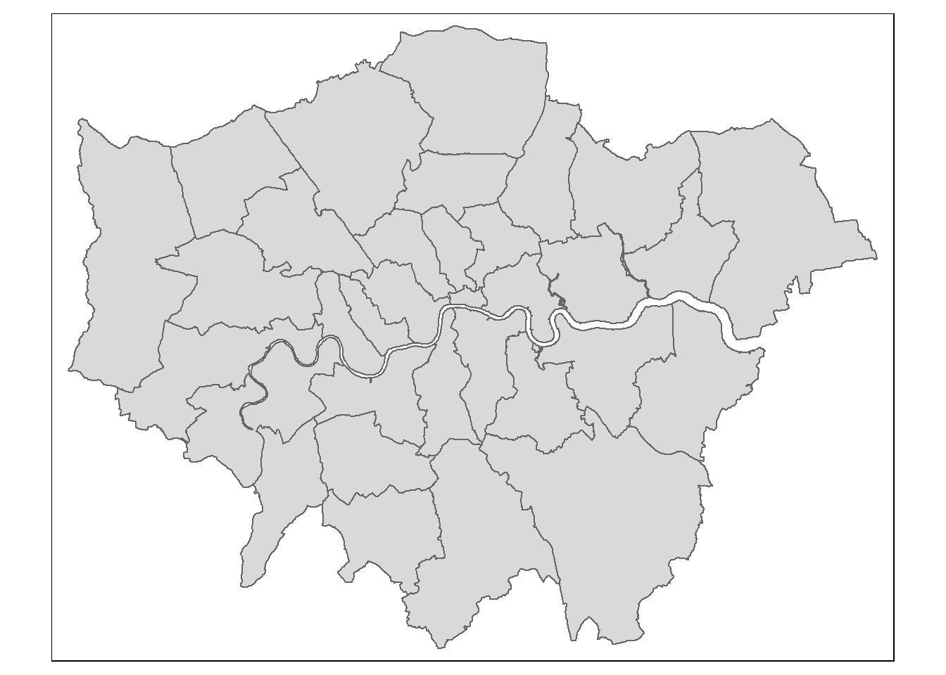
# Load LSOA shapefile
london_LSOA <- load_shapefile(url, "statistical-gis-boundaries-london/ESRI/LSOA_2011_London_gen_MHW.shp") %>%
st_transform(london_boroughs, crs = 4326)Reading layer `LSOA_2011_London_gen_MHW' from data source
`C:\Users\Andy\AppData\Local\Temp\Rtmpq2qcE4\file6c746ab25ef5\statistical-gis-boundaries-london\ESRI\LSOA_2011_London_gen_MHW.shp'
using driver `ESRI Shapefile'
Simple feature collection with 4835 features and 14 fields
Geometry type: MULTIPOLYGON
Dimension: XY
Bounding box: xmin: 503574.2 ymin: 155850.8 xmax: 561956.7 ymax: 200933.6
Projected CRS: OSGB36 / British National Gridtmap_options(check.and.fix = TRUE)
qtm(london_LSOA)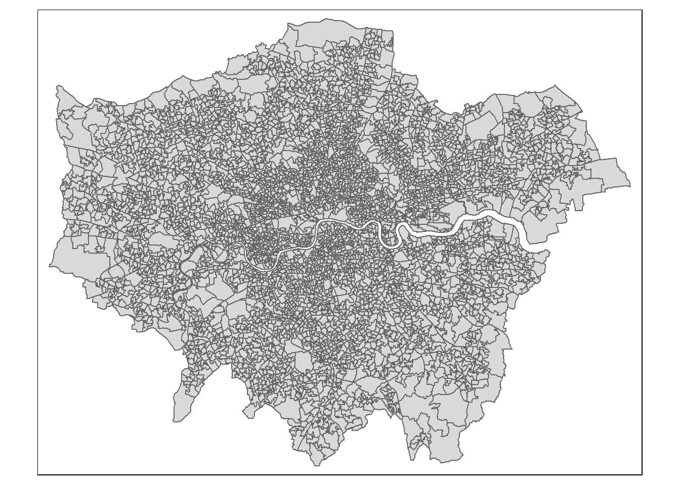
5.3.2 Download and read in the Index of Multiple Deprivation (IMD) data
#Load Index of Multiple Deprivation data. This can either be accessed from the CDRC website or downloaded directly from the government website.
#Downloaded data from the CDRC Index of Multiple Deprivation (IMD) website: https://data.cdrc.ac.uk/dataset/index-multiple-deprivation-imd/resource/data-english-imd-2019
#English IMD 2019. 2011 LSOA geography. Shapefile format.
#IMD_London <- st_read(here::here("data","English IMD 2019", "IMD_2019.shp")) %>%
# clean_names()%>%
# dplyr::filter(str_detect(la_dcd, "^E09"))
IMD_London <- st_read("https://services-eu1.arcgis.com/EbKcOS6EXZroSyoi/arcgis/rest/services/Indices_of_Multiple_Deprivation_(IMD)_2019/FeatureServer/0/query?outFields=*&where=1%3D1&f=geojson") %>%
st_transform(27700) %>%
clean_names() %>%
dplyr::filter(str_detect(la_dcd, "^E09"))Reading layer `OGRGeoJSON' from data source
`https://services-eu1.arcgis.com/EbKcOS6EXZroSyoi/arcgis/rest/services/Indices_of_Multiple_Deprivation_(IMD)_2019/FeatureServer/0/query?outFields=*&where=1%3D1&f=geojson'
using driver `GeoJSON'
Simple feature collection with 32844 features and 66 fields
Geometry type: MULTIPOLYGON
Dimension: XY
Bounding box: xmin: -6.418524 ymin: 49.86474 xmax: 1.762942 ymax: 55.81107
Geodetic CRS: WGS 84#Plot to see IMD deciles and check if all is correct
tmap_options(check.and.fix = TRUE)
tmap_mode("plot")
#Plot map
map <- tm_shape(IMD_London) +
tm_polygons(col = "imd_decile",
style = "pretty",
n = 10,
palette = "RdYlBu",
title = "IMD Decile",
border.alpha = 0) +
tm_layout(legend.position = c("right", "bottom"))
# +
# tm_shape(lnd_ff_pts) +
# tm_dots(col = "black",
# size = 0.05,
# border.lwd = 0,
# title = "Fast-food outlets", # Label for the dots
# legend.show = TRUE)
map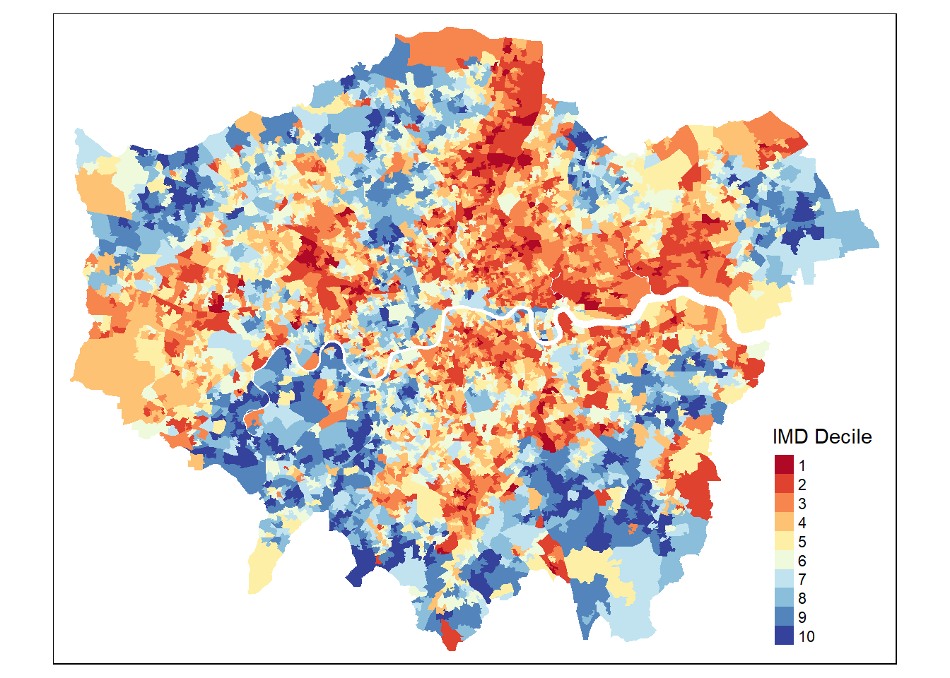
5.3.3 Load Fast-food points from Open Street Map (OSM)
As mentioned in the lecture, Open Street Map (OSM) is a great source of geospatial data. Here we will use the osmdata package to query OSM for fast-food outlets in London.
Later on in the practical we will ask you to find alternative points to analyse. Knowing what to search for can be a bit tricky, but the osmdata package has a function called available_features() which can be used to search for different types of points of interest. You can also use the available_tags() function to search for tags related to amenities.
You can also visit the OSM wiki to find out more about the different types of features and tags available - https://wiki.openstreetmap.org/wiki/Map_features or indeed, the main OSM page - https://www.openstreetmap.org/#map=13/51.49656/-0.05897
The osmdata package uses the Overpass Turbo API, which an also be used directly to download data here - https://overpass-turbo.eu/
# Load the required libraries
# Load the required libraries
library(DT)
features <- available_features() # Search for features in London
tags <- available_tags("amenity") # Search for tags related to amenities
tags_df <- data.frame(
Tag = tags, # Add the tags directly to the 'Tag' column
Description = NA # Placeholder column for descriptions (optional)
)
# Display the data frame as a DT table
datatable(
tags_df,# Select only the first 5 rows
options = list(pageLength = 10), # Display 5 rows
rownames = FALSE
)Using the feature tags in OSM, we can download data on fast food outlets directly.
# Define the geographic area (example: Greater London)
Bounding_box <- getbb("Greater London") # Bounding box for London
# Query OSM for fast food locations
fast_food <- opq(Bounding_box) %>%
add_osm_feature(key = "amenity", value = "fast_food") %>%
osmdata_sf()
# Extract point locations (fast food outlets)
fast_food_points <- fast_food$osm_points %>%
st_transform(4326) %>%
mutate(opps = 1)
# View first few rows
#head(fast_food_points)
#Filter out the points outside of our study area
fast_food_points <- fast_food_points[london_boroughs,]
# Plot fast food outlets
#plot(st_geometry(fast_food_points), col = "red", pch = 20, main = "Fast Food Outlets in London")
tmap_mode("plot")
map <- tm_shape(fast_food_points) +
tm_dots(col = "black",
size = 0.05,
border.lwd = 0,
title = "Fast-food outlets", # Label for the dots
legend.show = TRUE)
map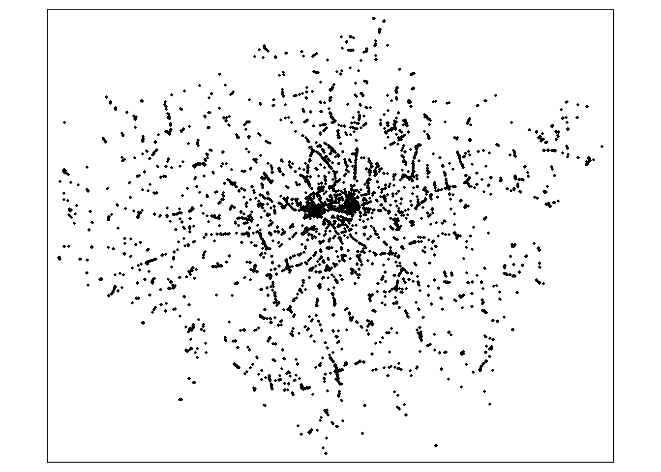
5.4 Load school points from Open Street Map (OSM)
School data are also available on OSM, however the tags are not that useful for distinguishing between different types of schools. The amenity tag can be used to search for schools, but this will return all types of schools (e.g., primary, secondary, etc.).
Primary schools can be filtered in London with the isced:level tag, but this is not always available. We will show you how to get the schools from OSM, but below we we also use an alternative method for accessing point data.
5.4.0.1 Bonus Extra Task - not required
See if you can think of a way of filtering out secondary schools from the tags available in OSM - you may need to use the filter() function in R to do this.
# Define the geographic area (example: Greater London)
Bounding_box <- getbb("Greater London") # Bounding box for London
# Query OSM for school locations
schools <- opq(Bounding_box) %>%
add_osm_feature(key = c("amenity"), value = "school") %>%
osmdata_sf()
# Extract point locations (schools)
schools_points <- schools$osm_points %>%
st_transform(4326) %>%
mutate(opps = 1)
# View first few rows
#head(schools_points)
#Filter out the schools outside of our study area
schools_points <- schools_points[london_boroughs,]
# Plot schools
#plot(st_geometry(schools_points), col = "blue", pch = 20, main = "Schools in London")
tmap_mode("plot")
map <- tm_shape(schools_points) +
tm_dots(col = "black",
size = 0.05,
border.lwd = 0,
title = "All Schools London", # Label for the dots
legend.show = TRUE)
map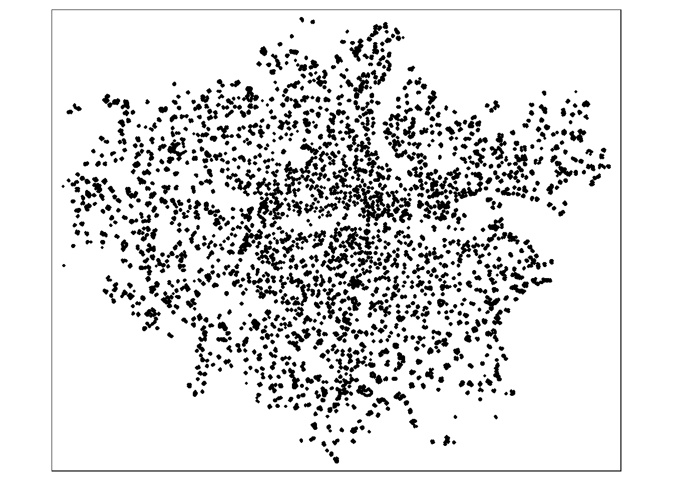
5.4.1 Alternative Method for Accessing School Points
Alternatively, the Department for Education’s Edubase database contains information for all schools - https://get-information-schools.service.gov.uk/ - here we read that data in and filter for secondary schools in London.
The crucial thing to note here is that the data is in British National Grid format, so we may need to transform it to WGS84 (EPSG 4326) to match the other data we have. However, we know it is in British National Grid as the data contains two columns - “easting” and “northing” - which is the standard way of referencing x and y coordinates in our projected coordinate reference system.
In the code below, we use the st_as_sf() function to convert the data to an sf object, and then the st_set_crs() function to set the coordinate reference system to British National Grid (EPSG 27700).
We are downloading and processing the data in one block, however, if you are not familiar with the column headers and the data contained in a file, always download and open it in excel first to get a sense of the contents.
london_sec_schools <- read_csv("https://www.dropbox.com/scl/fi/fhzafgt27v30lmmuo084y/edubasealldata20241003.csv?rlkey=uorw43s44hnw5k9js3z0ksuuq&raw=1") %>%
clean_names() %>%
filter(gor_name == "London") %>%
filter(phase_of_education_name == "Secondary") %>%
filter(establishment_status_name == "Open") %>%
st_as_sf(., coords = c("easting", "northing")) %>%
st_set_crs(27700)
schools_points <- london_sec_schools
tmap_mode("view")
map <- tm_shape(schools_points) +
tm_dots(col = "black",
size = 0.05,
border.lwd = 0,
title = "All Schools London", # Label for the dots
legend.show = TRUE)
map5.5 Creating Point Pattern Process (PPP) Objects
In order to carry out spatial point pattern analysis, we need to convert our spatial data into point pattern objects. We will use the spatstat package to create point pattern objects from our fast-food and school locations. We also need to make sure that all of our coordinates are in British National Grid (EPSG 27700) - a Projected Coordinate Reference System (CRS) for the UK as spatstat requires will not work on geographic coorinate systems like wgs84 (CRS: 4326).
Create some Point Pattern Process objects:
# Project schools and fast food outlets to British National Grid CRS
lnd_sch_bng <- st_transform(schools_points, 27700)
lnd_ff_bng <- st_transform(fast_food_points, 27700)
lnd_bng <- st_transform(london_boroughs, 27700)
# Summarize the transformed school points
#summary(lnd_sch_bng)
# Convert schools and fast food locations to PPP objects for spatial analysis
lnd_sch_ppp <- as.ppp(lnd_sch_bng)
lnd_ff_ppp <- as.ppp(lnd_ff_bng)
# Remove marks (attributes) from the PPP objects
marks(lnd_sch_ppp) <- NULL
marks(lnd_ff_ppp) <- NULL
# Convert London borough boundaries to observation window format
lnd_owin <- as.owin(lnd_bng)
# Assign the observation window to the fast food PPP object
Window(lnd_ff_ppp) <- lnd_owin
# Plot the fast food point pattern objects
plot(lnd_ff_ppp)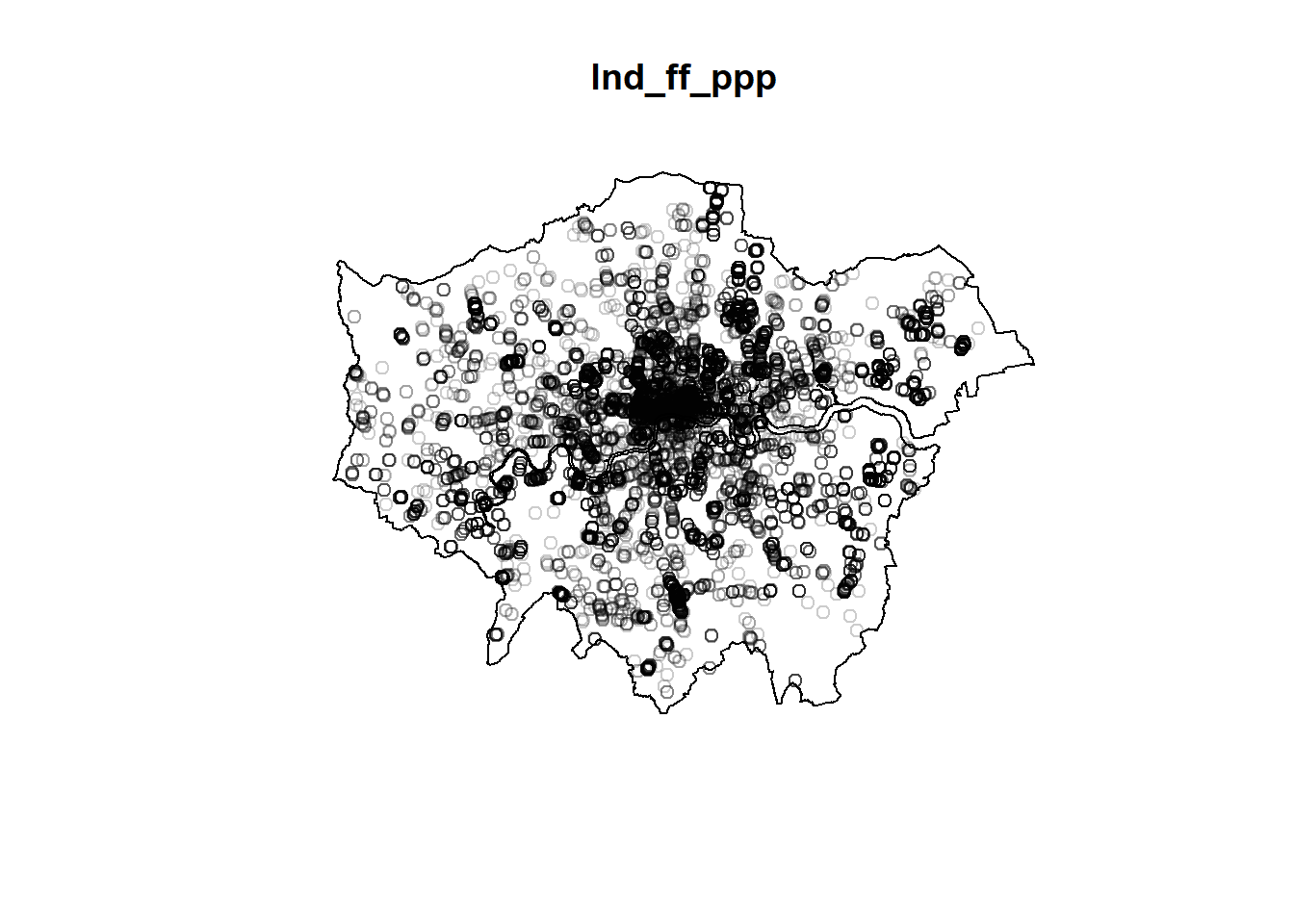
5.6 IMD (Index of Multiple Deprivation) Analysis
The aim of this analysis is to investigate whether areas with higher levels of deprivation have a greater density of fast-food outlets. This will help us determine if there are inequalities in fast-food outlet distribution based on area level deprivation - and if so, in which areas public health interventions should be prioritised.
5.6.1 Creating a Raster from IMD Data
# Convert the IMD shapefile into a raster format for analysis
IMD_London_raster <- st_rasterize(IMD_London %>% dplyr::select(imd_decile, geometry))
# Plot the generated raster
plot(IMD_London_raster)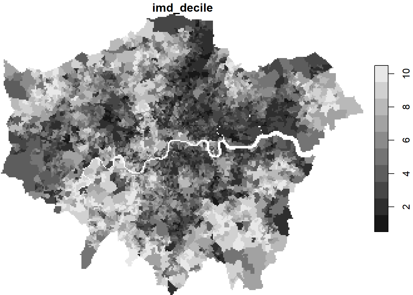
# Convert the raster to an IM object for statistical analysis
IMD_London_im <- as.im(IMD_London_raster)
# Plot the IM object
plot(IMD_London_im)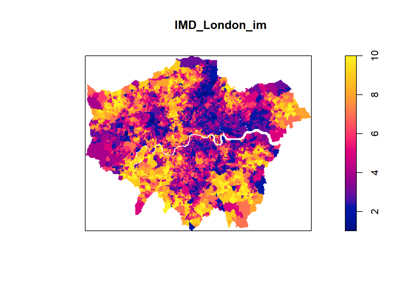
5.6.2 Quadrat Analysis on Fast Food Locations
We can carry out a quadrat count analysis to assess the spatial distribution of fast-food outlets in relation to area level deprivation. As you saw in previous practicals on this course, usually a quadrat analysis divides the study area into a grid of equal-sized squares (quadrats) and counts the number of points in each quadrat. Here we use IMD deciles as our ‘quadrat’ areas in exactly the same way. The quadrat count analysis can help us determine if fast-food outlets are clustered, dispersed, or randomly distributed in areas with different levels of deprivation.
# Set up the graphical parameters for a better layout
par(mar = c(4, 4, 2, 2)) # Adjust margins for visualization
dev.new() # Open a new plotting window to visualize the quadrat analysis
# Perform quadrat count analysis to assess spatial distribution
quad_ff_IMD <- quadratcount(lnd_ff_ppp, tess = IMD_London_im)
# Display quadrat count results
quad_ff_IMDtile
1 2 3 4 5 6 7 8 9 10
272 2466 2787 2249 1703 1390 1462 904 935 295 #test if significant clustering
chisq.test(quad_ff_IMD)
Chi-squared test for given probabilities
data: quad_ff_IMD
X-squared = 4709.2, df = 9, p-value < 2.2e-16# Plot the quadrat count analysis
plot(quad_ff_IMD)
5.6.2.1 Question - What does the quadrat analysis tell you about the spatial distribution of fast-food outlets in relation to area level deprivation?
5.7 Density Estimation with Rho-Hat Plot
As we saw in the lecture, we can take our analysis a little further by estimating the intensity of fast-food outlets across different levels of deprivation. The rho-hat function in spatstat estimates the intensity of point patterns as a continuous function of a covariate (rather than a discrete class).
# Generate and plot the rho-hat function to assess intensity variation by area level deprivation
plot(rhohat(lnd_ff_ppp, IMD_London_im))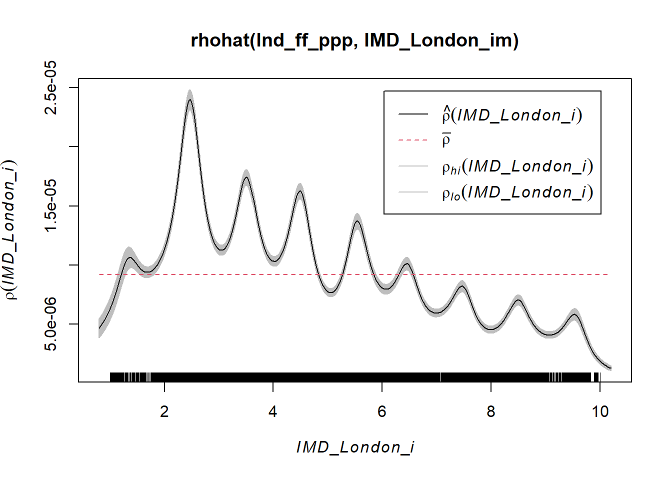
5.7.0.1 Question - What does the rho-hat plot tell you about the intensity of fast-food outlets across different levels of deprivation?
5.7.0.2 Question - why do you think this plot has a series of peaks and troughs?
In the above plot we used IMD deciles to explore the intensity of fast-food outlets across different levels of deprivation. The IMD, however, has a raw score associated with it as well that we can examine
# Convert the IMD shapefile into a raster format for analysis
imd_ldn_score_raster <- st_rasterize(IMD_London %>% dplyr::select(imd_score, geometry))
# Plot the generated raster
#plot(imd_ldn_score_raster)
# Convert the raster to an IM object for statistical analysis
IMD_ldn_score_im <- as.im(imd_ldn_score_raster)
# Plot the IM object
plot(IMD_ldn_score_im)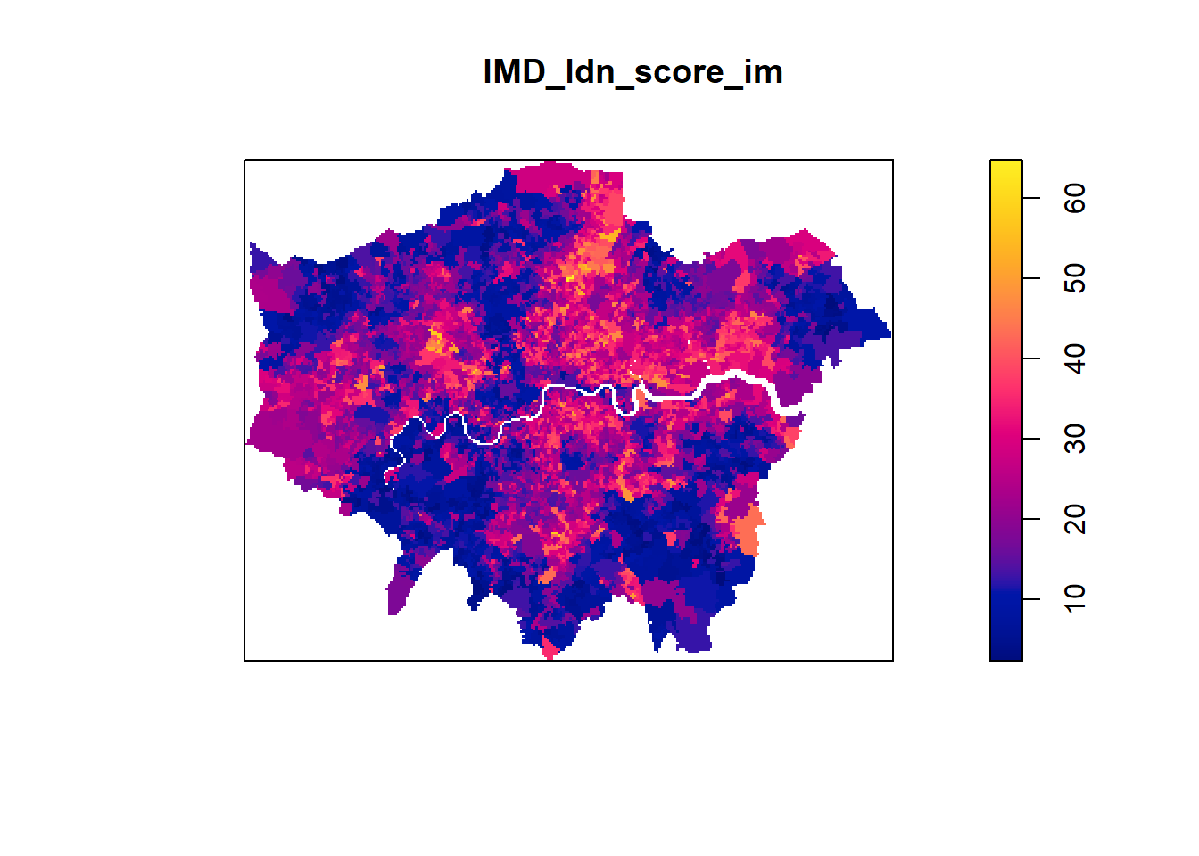
plot(rhohat(lnd_ff_ppp, IMD_ldn_score_im))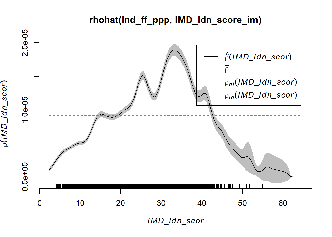
6 Part 2 - Extending Spatial Point Pattern Analysis in the presence of a covariate (buffers around schools)
The aim of this analysis is to determine which radius from schools captures the highest density of fast-food outlets. This will help us answer the question “How big should school fast-food exclusion zones be to cover areas of greatest exposure for school children?”
There are different ways in which we can create buffers around schools. One way is to use the st_buffer() function from the sf package. This function creates a buffer around a set of points, lines, or polygons. The buffer distance can be specified in meters, kilometers, or any other unit of measurement. There is some hidden code above which will do this, however, these buffers are not rasterized and so cannot be used in the analysis below.
To create a distance surface, we can use the distance() function from the terra package. This function calculates the distance from each cell in a raster to the nearest cell in a set of points. The resulting distance surface can be used to calculate the distance from each cell in the raster to the nearest school. This distance surface can then be used to create buffers around the schools.
It’s quite important not to set your resolution too high, as this can lead to memory issues if you have a large are (like London). Below we set the resolution to 100m square grid cells, but you may need to adjust this depending on the size of the area you are working with and the resolution that makes sense.
# Load necessary libraries
library(sf)
library(dplyr)
library(terra)
# Convert your sf points to a SpatVector
schools_vect <- vect(schools_points)
# Create a base raster grid (adjust resolution as needed)
r <- rast(ext(schools_vect), resolution = 100, crs = crs(schools_vect)) # Example: 100m resolution
# Create the distance surface
distance_surface <- distance(r, schools_vect)
# Cap the distances at 5000
distance_surface_capped <- clamp(distance_surface, lower = 0, upper = 2000)
# Plot the capped distance surface
plot(distance_surface_capped, main = "Distance Surface (Capped at 2km)")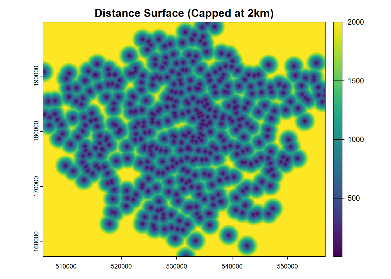
#tmap_mode("view")
#tm_shape(distance_surface_capped) +
# tm_raster("lyr.1", palette = "viridis", alpha = 0.5, title = "School Distance")
df <- as.data.frame(distance_surface_capped,xy=TRUE)
school_distance.im <- as.im(df)
class(school_distance.im)[1] "im"plot(school_distance.im) 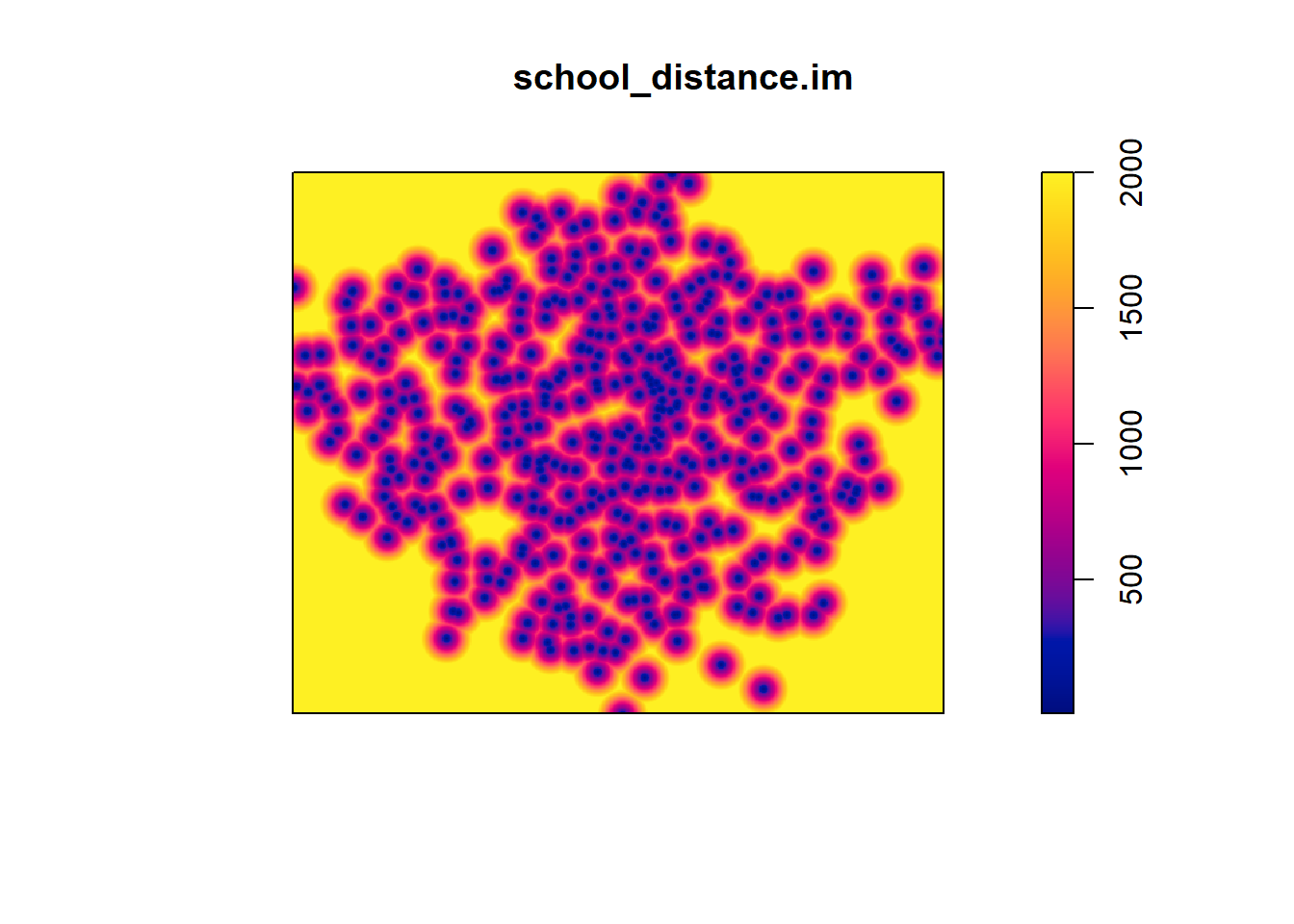
plot(rhohat(lnd_ff_ppp, school_distance.im))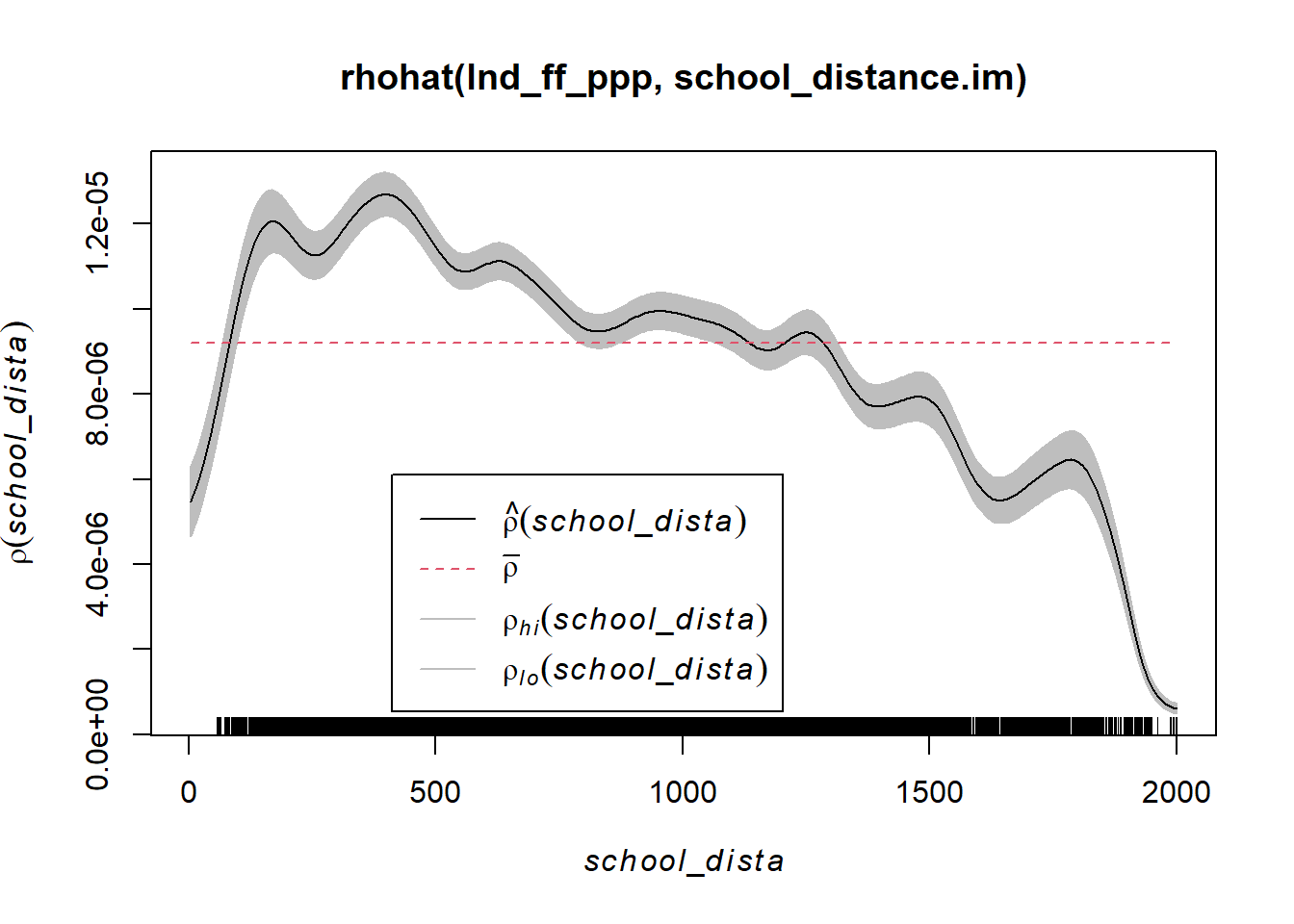
6.0.0.1 Question - What does the rho-hat plot tell you about the intensity of fast-food outlets across different distances from schools?
7 Part 3 - Find and Analyse Alternative Point Data
In this part of the practical, we would like you to find alternative point data from Open Street Map (or other sources - these road traffic collision data might be interesting too - https://tfl.gov.uk/corporate/publications-and-reports/road-safety#on-this-page-2) which may either have alternative health impacts, good or bad. We would like to you to apply the analysis methods you have learned above to this new data and think about the following questions as you do so:
What is the spatial distribution of the new point data? Are there methods from earlier in the course that you could use to get a sense of whether your data are dispersed or clustered, for example?
Are there any covariates (other than the ones we have already used) that you could use to investigate the spatial distribution of the new point data?
What are the implications of the spatial distribution of the new point data for public health (or any other) policy?
What are the limitations of the analysis you have carried out? Are there any other methods you have learned you could use to investigate the spatial distribution of the new point data that would make sense?
Can you think of any other data or contexts where these methods might be useful?
8 Extension Activity - Extending Spatial Point Pattern Analysis in the presence of a covariate (walking time bands) using R5 accessibility analysis
This is an extension activity that you do not have to complete as the r5r package can provide problematic to install due to its java development kit requirements. However, if you are able to install the package, the code below will show you how to use the R5 accessibility analysis tool to calculate travel times from schools to fast-food outlets.
For guidance on how to install and use r5r - please visit the excellent documentation pages here - https://ipeagit.github.io/r5r/
The aim of this extension is to determine the walking distance from schools that captures the highest density of fast-food outlets. This will help us answer the question “Within what walking distance from schools are children the most exposed to fast-food outlets?” We are going to do this for a single London borough for the purpose of this exercise (the borough of Croydon)
8.1 Setup R5 Environment
# give yourself a bit more memory
options(java.parameters = "-Xmx20G")
# Initialize Java Virtual Machine
rJava::.jinit()
rJava::.jcall("java.lang.System", "S", "getProperty", "java.version")
# Set memory allocation
# Load OpenStreetMap data for London
oe_match("London, England")
roads_london = oe_get("London, England", stringsAsFactors = FALSE, quiet = TRUE)
names(roads_london)
#summary(roads_london)
# Filter major road types
ht = c("motorway", "trunk", "primary", "secondary", "tertiary", "residential", "unclassified")
osm_London_maj_roads = roads_london[roads_london$highway %in% ht, ]
#plot(osm_London_maj_roads["highway"], key.pos = 1)
#plot(sf::st_geometry(roads_london))
osm_download <- list.files(oe_download_directory())
osm_file <- paste0(oe_download_directory(),"\\","geofabrik_greater-london-latest.osm.pbf")
file.copy(from=osm_file, to=here(),
overwrite = TRUE, recursive = FALSE,
copy.mode = TRUE)
# Setup R5 transport network
here()
r5r_core <- setup_r5(here())8.2 Reproject Data to a Consistent CRS (EPSG 4326)
# Convert spatial data to EPSG 4326
school_points_EPSG <- schools_points %>%
st_transform(4326) %>%
mutate(opps = 1) %>%
mutate(id = row_number())
fastfood_points_EPSG <- fast_food_points %>%
st_transform(4326) %>%
mutate(opps = 1)
london_boroughs_EPSG <- london_boroughs %>%
st_transform(4326)8.3 Filter Data for the Borough of Croydon Only
# Extract Croydon boundary
croydon <- london_boroughs_EPSG %>%
filter(GSS_CODE == "E09000008")
# Extract Croydon-specific school and fast food locations
croydon_sch_pts <- school_points_EPSG[croydon,]
croydon_ff_pts <- fastfood_points_EPSG[croydon,]8.4 Generate Hexagonal Grid for Croydon
croydon_h3 <- polygon_to_cells(croydon, res = 11, simple = FALSE)
croydon_h3 <- cell_to_polygon(unlist(croydon_h3$h3_addresses), simple = FALSE)
croydon_h3_centroids <- st_centroid(croydon_h3)
# Summarize and visualize the hexagonal grid
#summary(croydon_h3)
# ggplot() +
# geom_sf(data = croydon, fill = NA) +
# geom_sf(data = croydon_h3, fill = NA, colour = 'red') +
# ggtitle('Resolution 10 hexagons', subtitle = 'Croydon') +
# theme_minimal() +
# coord_sf()
tm_shape(croydon) +
tm_polygons(col = "red", alpha = 0) +
tm_shape(croydon_h3) +
tm_polygons(col = NA, alpha = 0) +
tm_shape(croydon_ff_pts) +
tm_dots(col = "blue", border.lwd = 0) +
tm_shape(croydon_sch_pts) +
tm_dots(col = "black", border.lwd = 0) 8.5 Travel Time Matrix Calculation
# Prepare data for travel time calculations
croydon_sch = croydon_sch_pts %>% st_drop_geometry()
croydon_h3_centroids[c("x", "y")] = st_coordinates(croydon_h3_centroids)
# Assign IDs
croydon_h3_centroids <- mutate(croydon_h3_centroids, id = row_number())
croydon_h3 <- mutate(croydon_h3, id = row_number())
# Define travel parameters
mode = c("WALK")
max_walk_time = 30 # Maximum walking time in minutes
max_trip_duration = 120 # Maximum trip duration in minutes
departure_datetime = as.POSIXct("01-12-2022 8:30:00", format = "%d-%m-%Y %H:%M:%S")
# Compute travel time matrix
ttm_croydon_h3 = travel_time_matrix(
r5r_core = r5r_core,
origins = croydon_sch_pts,
destinations = croydon_h3_centroids,
mode = mode,
departure_datetime = departure_datetime,
max_walk_time = max_walk_time,
max_trip_duration = max_trip_duration
)
#head(ttm_croydon_h3)
#nrow(ttm_croydon_h3)
#summary(ttm_croydon_h3)8.6 Identify Closest Schools by Travel Time
# Find minimum travel time per destination
closest = aggregate(ttm_croydon_h3$travel_time_p50, by = list(ttm_croydon_h3$to_id), FUN = min, na.rm = TRUE)
summary(closest)
# Rename columns
closest <- rename(closest, id = Group.1, time = x)
closest["id"] = as.integer(closest$id)
head(closest)
# Join spatial data with travel time results
geo = inner_join(croydon_h3_centroids, closest, by = "id")
geo_hex = inner_join(croydon_h3, closest, by = "id")
head(geo)8.7 Visualizing Travel Time Data
tm_shape(geo) +
tm_symbols(col = "time", size = 0.05, border.lwd = 0, style = "pretty", n = 10, palette = "RdYlBu", alpha = 0.3) +
tm_shape(croydon_sch_pts) +
tm_dots(col = "black", border.lwd = 0) +
tm_shape(croydon) +
tm_polygons(alpha = 0)8.8 Convert Data to British National Grid (EPSG 27700) and Analyse Spatial Distribution
# Reproject spatial data
geo_hex_bng <- st_transform(geo_hex, 27700)
# Convert raster data
raster_geo <- st_rasterize(geo_hex_bng %>% dplyr::select(time, geometry))
st_coordinates(raster_geo)
plot(raster_geo, axes = T)
geo_hex_im <- as.im(raster_geo)
plot(geo_hex_im)8.9 Quadrat Analysis of Fast Food Locations
# Convert to spatial point pattern objects
croy_sch_bng <- st_transform(croydon_sch_pts, 27700)
croy_ff_bng <- st_transform(croydon_ff_pts, 27700) %>%
select(c("osm_id", "name", "geometry"))
croydon_bng <- st_transform(croydon, 27700)
croy_ff_ppp <- as.ppp(croy_ff_bng)
croydon_owin <- as.owin(croydon_bng)
Window(croy_ff_ppp) <- croydon_owin
# Quadrat count analysis
Q <- quadratcount(croy_ff_ppp, nx= 6, ny=6)
plot(croy_ff_ppp, pch=20, cols="grey70", main=NULL); plot(Q, add=T)8.10 Spatial Density Analysis
plot(rhohat(croy_ff_ppp, geo_hex_im))8.11 Kolmogorov-Smirnov Test for Spatial Distribution
ks_result <- cdf.test(croy_ff_ppp, "x")
print(ks_result)