Practical 1 – Geographic Information
In your N drive: drive, create a new folder called GIS and within this a subfolder called wk1
1 Learning outcomes
By the end of this practical you should be able to:
- Describe and explain GIS data formats and databases
- Source and pre-process spatial data
- Load and undertaken some basic manipulcation of spatial data in: ArcMap, QGIS and R
- Evaluate the (dis)advantages of each GIS you have used
2 The Basics of Geographic Information
Geographic data, geospatial data or geographic inforamtion is data that identifies the location of features on Earth. There are two main types of data which are used in GIS applications to represent the real world. Vectors – points, lines and polygons and rasters – grids of cells with individual values.
 Real world
  Raster
  Vector
In the above example the features in the real world (e.g. lake, forest, marsh and grassland) have been represented by points, lines and polygons (vector) or discrete grid cells (raster) of a certain size (e.g. 1 x 1m) specifying land cover type.
2.1 Important GIS data formats
There are a number of commonly used geographic data formats that store vector and raster data that you will come across during this course and it’s important to understand what they are, how they represent data and how you can use them.
2.1.1 Shapefiles
Perhaps the most commonly used GIS data format is the shapefile. Shapefiles were developed by ESRI (http://www.esri.com/) – one of the first and now certainly the largest commercial GIS company in the world. Despite being developed by a commercial company, they are an open format and Shapefiles can be used (read and written) by a host of GIS Software applications.
A shapefile is actually a collection of files – at least three of which are needed for the shapefile to be displayed by GIS software. They are:
.shp- the file which contains the feature geometry.shx- an index file which stores the position of the feature IDs in the .shp file.dbf- the file that stores all of the attribute information associated with the coordinates – this might be the name of the shape or some other information associated with the feature.prj- the file which contains all of the coordinate system information (the location of the shape on Earth’s surface). Data can be displayed without a projection, but the.prjfile allows software to display the data correctly where data with different projections might be being used
2.1.2 GeoJSON
GeoJSON (Geospatial Data Interchange format for JavaScript Object Notation, http://geojson.org/) is becoming an increasingly popular spatial data format, particularly for web-based mapping as it is based on JavaScript Object Notation. Unlike a shapefile in a GeoJSON the attributes, boundaries and projection information are all contained in the same file.
2.1.3 Shapefile and GeoJSON
We’re now going to explore a shapefile (.shp ) and GeoJSON (.geojson) in action.
Go to: http://geojson.io/#map=16/51.5247/-0.1339
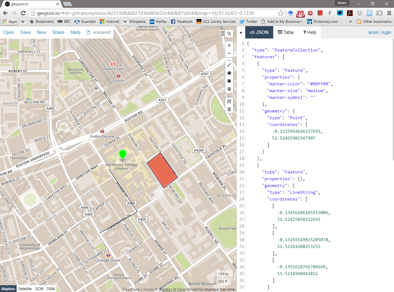
- Using the drawing tools to the right of the map window, create 3 objects: a point, line and a polygon as I have done above. Click on your polygon and colour it red and colour your point green.
- Using the ‘Save’ option at the top of the map, save two copies of your new data – one in
.geojsonformat and one in.shpformat. - Open your two newly saved files in a text editor such as notepad or notepad++. For the shapefile you might have to unzip the folder then open each file individually. What do you notice about the similarities or differences between the two ways that the data are encoded?
2.1.4 Raster data
Most raster data is now provided in GeoTIFF (.tiff) format, which stands for Geostarionary Earth Orbit Tagged Image File. The GeoTIFF data format was created by NASA and is a standard public domain format. All necesary inforamtion to establish the location of the data on Earth’s surface is embedded into the image. This includes: map projection, coordinate system, ellipsoid and datum type.
2.1.5 Other data formats
Aforementioned data types and formats are likely to be the ones you predominately encounter. However there are several more used within spatial analysis. Theres include:
Vector
- GML (Geography Markup Language – gave birth to KML) - http://www.opengeospatial.org/standards/gml
Raster
- Band SeQuential (BSQ) - technically a method for encoding data but commonly refered to as BSQ.
- Hierarchical Data Format (HDF)
- Arc Grid
There are normally valid reasons for storing data in one of these other formats. For example, BSQ are raster data with a seperate text header file (.hdr) providing geographic spatial reference information. Earth observation data often monitors the electromagenitc spectrum in bands. Humans see in the visible range of the spectrum and our vision is composed of red, green and blue wavelengths. If we wanted to analyse just the red wavelength the BSQ format would let us read in only that data. In comaprsion a GeoTIFF might come with all the data ‘packaged’ in one file and when doing analysis over thousands of images would significantly slow things down. That said you can now often find GeoTIFFs seperated in a similar format to BSQ and it’s fairly straightforward to convert between raster formats. Often the most successful projects and reports will combine numerous datasets from various sources (and in different formats) to glean new insights.
2.1.6 Geodatabase
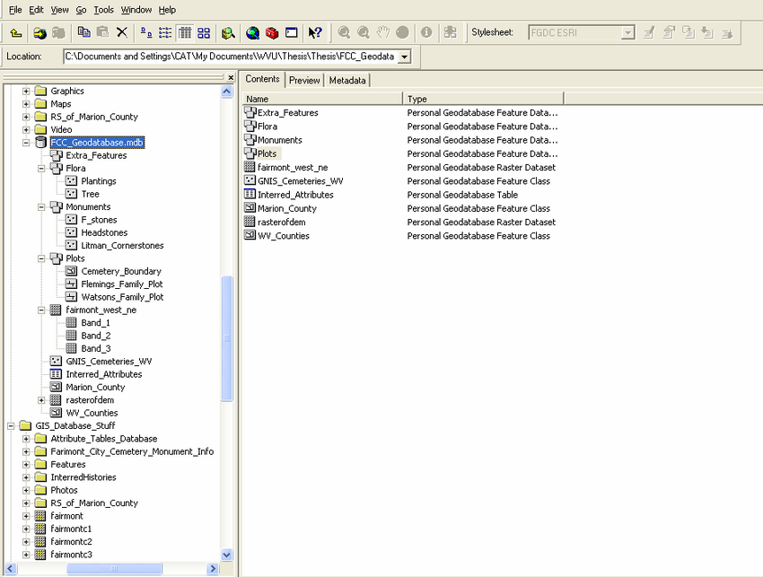
A geodatabase is a collection of geographic data held within a database. Geodatabases were developed by ESRI to overcome some of the limitations of shapefiles. They come in two main types: Personal (upto 1 TB) and File (limited to 250 - 500 MB), with Personal Geodatabases storing everything in a Microsoft Access database (.mdb) file and File Geodatabases offering more flexibility, storing everything as a series of folders in a file system. In the example below we can see that the FCC_Geodatabase (left hand pane) holds multiple points, lines, polygons, tables and raster layers in the contents tab.
2.1.7 GeoPackage

A GeoPackage is an open, standards-based, platform-independent, portable, self-describing, compact format for transferring geospatial data. It stores spatial data layers (vector and raster) as a single file, and is based upon an SQLite database, a widely used relational database management system, permitting code based, reproducible and transparent workflows. As it stores data in a single file it is very easy to share, copy or move.
2.1.8 SpatiaLite
SpatialLite is an open source library that extends SQLite core. Support is fairly limited and most software that supports SpatiaLite also supports GeoPackage, as they both build upon SQLite. It doesn’t have any clear advantage over GeoPackage, however it is unable to support raster data.
2.1.9 PostGIS

PostGIS is an opensource database extender for PostrgeSQL. Essentially PostgreSQL is a database and PostGIS is an add on which permits spatial functions. The advantages of using PostGIS over a GeoPackage are that it allows users to access the data at the same time, can handle large data more efficiently and reduces processing time. In this example (https://medium.com/@GispoLearning/learn-spatial-sql-and-master-geopackage-with-qgis-3-16b1e17f0291) calcualting the number of bars per neighbourhood in Leon, Mexico the processing time reduced from 1.443 seconds (SQLite) to 0.08 seconds in PostGIS. However, data stored in PostGIS is much harder to share, move or copy.
2.1.10 What will I use
The variety of data formats can see a bit overwhelming. But don’t worry, most of the time you’ll be using shapefiles, GeoPackages or raster data.
3 Data
The volume of geographic information which is freely available for use in the UK is increasing exponentially and spatially referenced data can often be found in many different places. In this practical we’re going to use data from the London data store - a free and open data-sharing portal provided by the Greater London Authrotiy (GLA), also known as City Hall that is the devovled regional governance body of London.
We are going to get spatial data of the London boroughs and join flytipping (where rubbish is dumped illegally) data that is provided as a .csv file. .csv stands for comma-separated values (CSV) - it uses a comma to separate each value.
At the end of this document I’ll also run through some common sources of data that will stand you in good stead (be advantagous) for the rest of the course.
3.1 Data download
Firstly we need to get a spatial outline of the London boroughs. The geographic boundaries that are used in the UK are a complex, often inter-related, but ever changing mass of areas. For anyone new to the UK (or indeed not a trained quantitative geographer), it can be quite a daunting task to attempt to understand all of the boundaries that are in use. Fortunately the Office for National Statistics (ONS) has an online beginners guide to UK geography. If you need more information on the vast array of different UK geographies, this is the place to start: http://geoportal.statistics.gov.uk/datasets/a-beginners-guide-to-uk-geography-2018-v1-0
- Spatial Data
To get the data go to: https://data.london.gov.uk/
Seach for Statistical GIS Boundary Files for London
Download the statistical-gis-boundaries-london.zip
Unzip the data and save it to your week 1 folder.
- CSV data
On the same website search for fly-tipping incidents
Download the
.csvfile
3.2 Data pre-processing
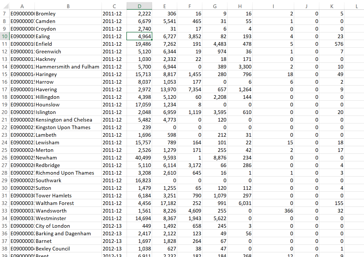
Question Open the .csv in Excel, what do you notice about how the data is stored?
Answer The year is a column and for each area the values are repeated for different years. In our analysis it is easier to have the different years as a coloumn and populated for each area. So, we want to go from this…
To this…
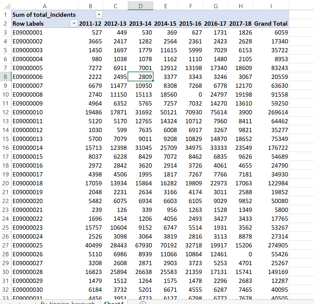
As we are going to use this dataset in ArcMap, QGIS and R I’ve done it in Excel using a pivot table.
Go to Insert > PivotTable
Select the original table and create a PivotTable in a new worksheet
The PivotTable Field box will appear, experiment with the different fields in each of the areas
I’ve used the following:
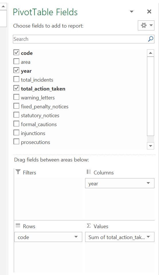 Note how I’ve altered the total_action_taken to the sum of… as the original was displaying incorrectly, to do so:
- Click on drop down button for total_action_taken > Value Field Settings > select Count
It’s important to think about what data we actually need in the next step and it’s good practice to avoid data redundancy where possible.
Spoiler - the spatial data we have downloaded already contains borough name, so we don’t need it twice. However, we do need a field to link the two datasets on. You could use borough name, but when using text fields sometimes input variations can affect joins. For example, you had the University of Manchester in one dataset and Manchester University in another the join would fail. Consequntly it’s usually best to join datsets on a code field.
Now save the Excel sheet that contains the pivot table as a new .csv. Make sure that the first row of data holds the coloumn titles. Remove all empty rows.
When saving the file also avoid any special characters (e.g. -) and spaces, use an underscore instead of spaces.
Warning spatial software (especially ArcGIS) does not like file names with spaces or special characters.
3.3 Data loading
Now it’s time to load, inspect and do some basic manipulation of this data. As mentioned in the lecture there are several GIS software ‘types’, here we will repeat the same process across ArcGIS, QGIS and R. Each system has specific benefits, but in general there has been a recent shift towards the use of QGIS and R, both being opensource. ArcGIS was the first major spatial analysis software produced by the Environmental Systems Research Institute, Inc. (Esri), founded in 1969 by Jack Dangermond. Due to its high cost and lack of customisation it is now less commonly used within the research community.

3.4 ArcGIS
3.4.1 Basics
ArcGIS should be installed as a standard programme in the UCL desktop and you should be able to navigate to it from the Windows start button.
3.4.1.1 Installing ArcGIS on your own computer
As a UCL student, you can install ArcGIS on your own computer. This is easy if you have a PC, but if you have a Mac this can be trickier as Arc will only run in a PC environment. If you have a Mac, the options open to you are either to:
- Run ArcGIS through the Desktop@UCL application - http://www.ucl.ac.uk/isd/services/computers/remote-access/desktop
- Duel boot your machine using bootcamp, install Windows (7 or 8 is fine) and then install Arc onto the Windows partition.
- Install some kind of virtualisation software such as Parallels (http://www.parallels.com/ca/products/desktop/) or VMware (http://www.vmware.com/products/fusion/), and run Arc on a virtual windows machine
If you can, it is preferable to run Arc on Bootcamp as virtualisation software can be slow, but the Desktop@UCL facility should suffice for this course. ArcGIS (Version 10.6 is the latest at time of writing, but may have already been superseded) can be downloaded from the UCL Software Database for free - https://swdb.ucl.ac.uk/.
3.4.1.2 Getting Help
ArcGIS is a huge and complex piece of software, but thankfully is has an excellent help system – depending on the version you are using (they are all quite similar anyway) you can access the online help system here:
3.4.1.3 ArcGIS
ArcGIS is actually a whole suite of software built and maintained by ESRI (http://www.esri.com/software/arcgis).Within the ArcGIS for Desktop suite you will find the following programmes:
ArcCatalog - Similar to Windows Explorer, ArcCatalog allows you to manage your GIS files, folders and geodatabases
ArcGIS Administrator - This programme us used to manage licences for the various elements of ArcGIS
ArcGlobe - ArcGlobe allows you to view and analyse your data in 3D – this interface looks very similar to Google Earth and is part of the 3D analyst extension
ArcMap - This is the programme you will use most often – it is the main mapping and spatial analysis element of ArcGIS
ArcScene - ArcScene is a 3D viewer which allows you to navigate and interact with your 3D raster and feature data
ArcCatalog and ArcMap are in bold as these are the only programmes we will be using explicitly in this course. By all means experiment with the others if you have any spare time!
3.4.2 ArcCatalog
Find and run the ArcCatalog piece of software
Once ArcCatalog Opens, go to File > Connect To Folder… and navigate to the N:folder, right click in the contents area and create a new Flie Geodatabase.
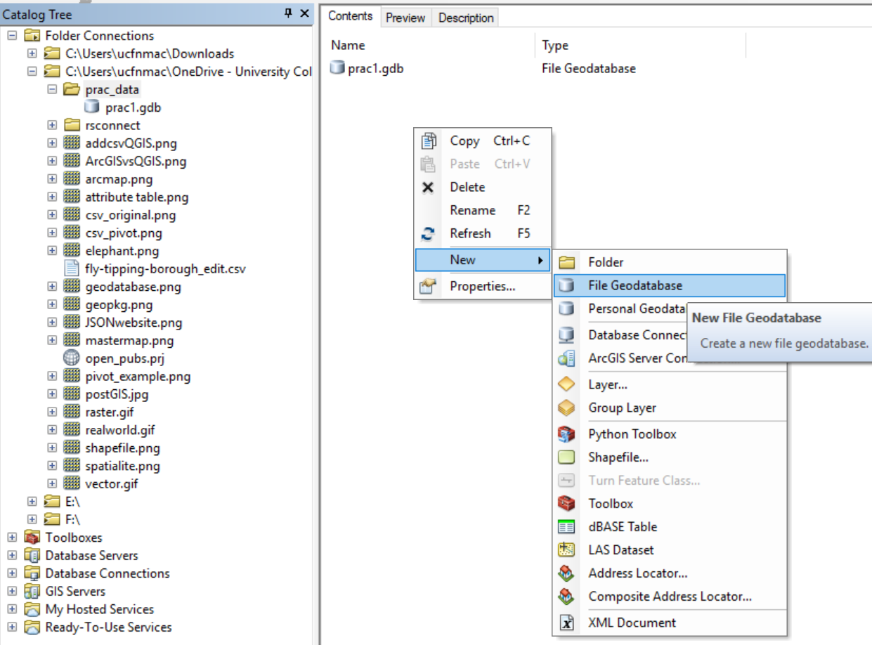
You can import data layers into a Geodatabase within ArCatalog, however we will do this in ArcMap.
3.4.3 ArcMap
3.4.3.1 Introduction
ArcMap is the core of the ArcGIS suite and where you would normally produce maps, carry out spatial analysis functions and automate processes.
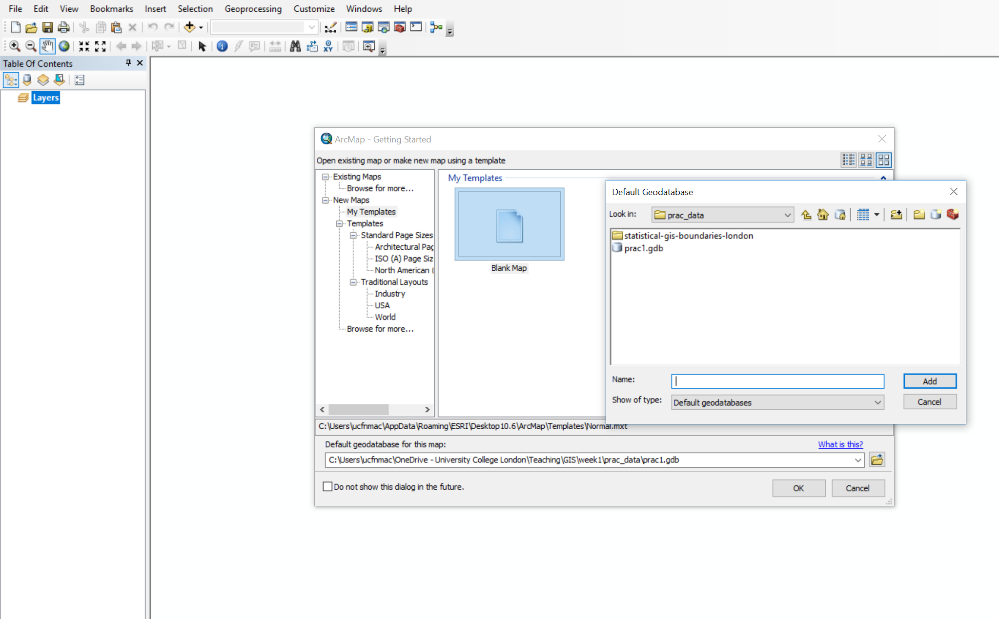
- Search for and open ArcMap
- Upon opening select the database you just created in the dialogue box
- Click ok
When the map document opens you should see something similar to the image below. ArcMap has various elements to the graphical user interface, but here some of the key buttons are highlighted:
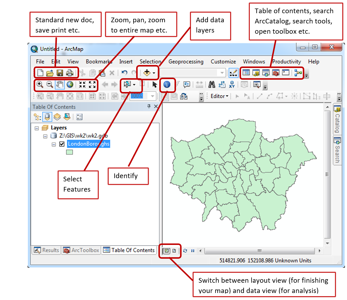
- It’s important to now set the map document up properly. Go File > Map Document Properties, enter the details you wish. You can see the connection to the Geodatabase we just made. Click store relative pathnames, this means as long as the data stays in the same position relative to the path then ArcMap can load all the layers. For example if you moved your work from the C: drive to an external drive, H:.
3.4.3.2 Load data
- Using the Plus icon (add data layer) navigate to the extracted folder you saved earlier.
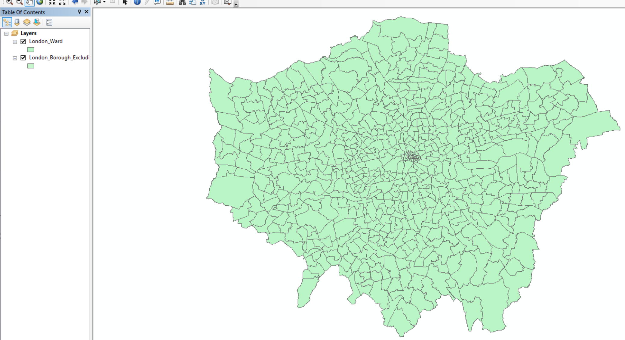
- Open London_Borough_Excluding_MHW.shp, but feel free to explore the other data layers. In the left hand Table Of Contents you can unselect layers to turn them off or drag layers above or below to change the display order. In the example below the wards layer is showing above the borough layer.
Note, while we have loaded the shapefile, it is not stored in our Geodatabase yet.
Useful tips
To the right of the document you will see the Catalog and Search tabs.The Catalog tab is a small version of ArcCatalog and will let you see what data is stored in the current Geodatabase. The search tab will let you find any analysis tool within ArcGIS. Try searching for Clip.
If you right click on the boroughs layer (in the Table of Contents, left hand pane) you will see various options. Zoom to layer is very useful if you ever get lost in your ArcMap document.
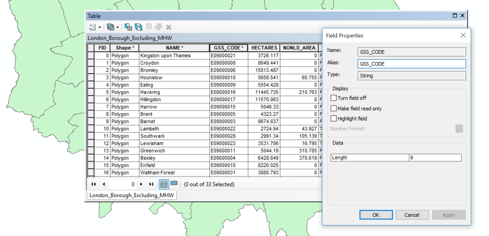
- Now right click on the borough layer (in the Table of Contents) and open the attribute table. You’ll see the GSS_CODE field, which is the same code we output in our
.csv. If you now right click on a field you’ll also be able to see the data type (e.g. string, integer). For example:
3.4.3.3 Join data
We’re now going to join our flytipping data to the lonon borough shapefile. So:
- Right click on the london borough layer > Joins and Relates > Join
- Select the GSS_CODE as the field in the layer to base the join on
- Navigate to the
.csvwe created earlier - Select the code field that matches (in my case this is called Row Labels)
- Select only to join matching records
- Validate join and click OK
You will get errors, ArcMap does not like fields starting with numbers (e.g. 2012), dashes (e.g. -) or spaces. Feel free to change them in the original .csv but for this practical it is fine to continue.
- The join should work, so reopen the attribute table for the layer london boroughs
Note, the join we have made is not permanent. To do so we need to export the layer.
3.4.3.4 Export data
- Right click on the london boroughs layer > Data > Export Data
- The location should default to our GeoDatabase. Be sure to change the filename - again avoid all of the characters (e.g. spaces and -) previously mentioned. Add the data layer to the map
Now lets use the data we’ve joined to create a basic thematic map.
- Right click on the new London borough layer > Properties
- Under the Symbology tab select Graduated colors
- Select the Value as one of the years of data we joined and change the classificaiton to something of your choice
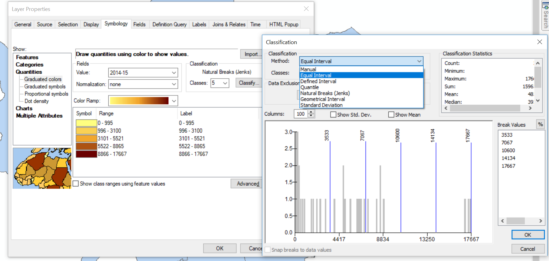
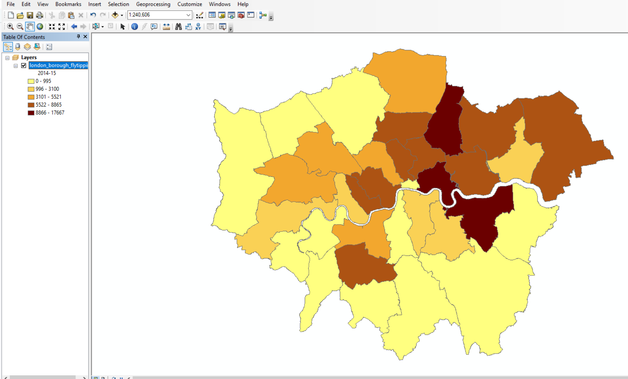
You should have something that looks like this:
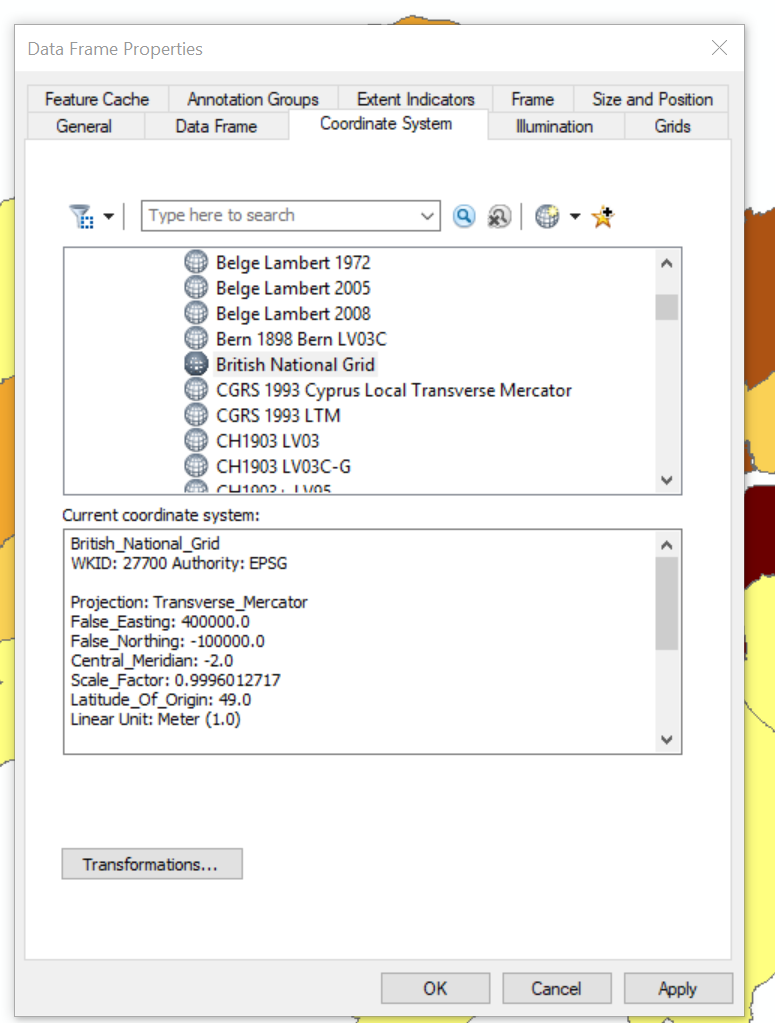
We haven’t talked about the Coordiante Reference System (CRS) (or Spatial Reference sSystem (SRS)) of our map document
A coordinate reference system is a series of paramters that define the coordinate system. Within GIS we use geographic or projected cooridnate systems. The former uses a three-dimesional spherical surface to define locations of earth, whereas the latter is defined on a flat, two-dimesional surface giving it constat lengths, angles and areas.
In ArcMap we can specify what CRS we want to use by:
- Right clicking on the map document > Data Frame Properties
You’ll see that it is already set to Projected Coordinate Systems, National Grids, Europe, British National Grid. This is because ArcMap will default to the cooridnate system of the first data layer loaded.
Save your ArcMap document. We’re now going to replicate this task in QGIS.
3.5 QGIS
3.5.1 Introduction
QGIS is very similar to ArcMap except that as it is open source and free there are many add on packages that (or plugins) that provide additional functionality to the software.
To get QGIS on your personal machine go to: https://qgis.org/en/site/forusers/download.html
I install the OSGeo4W version. The nature of open source means that several programs will rely on each other for features. OSGeo4W tracks all the shared requirements and does not intall any duplicates.
3.5.2 Load data
- Search for and open QGIS
- Click on the open data source manager. Just above the word browser in the top left of the screen.
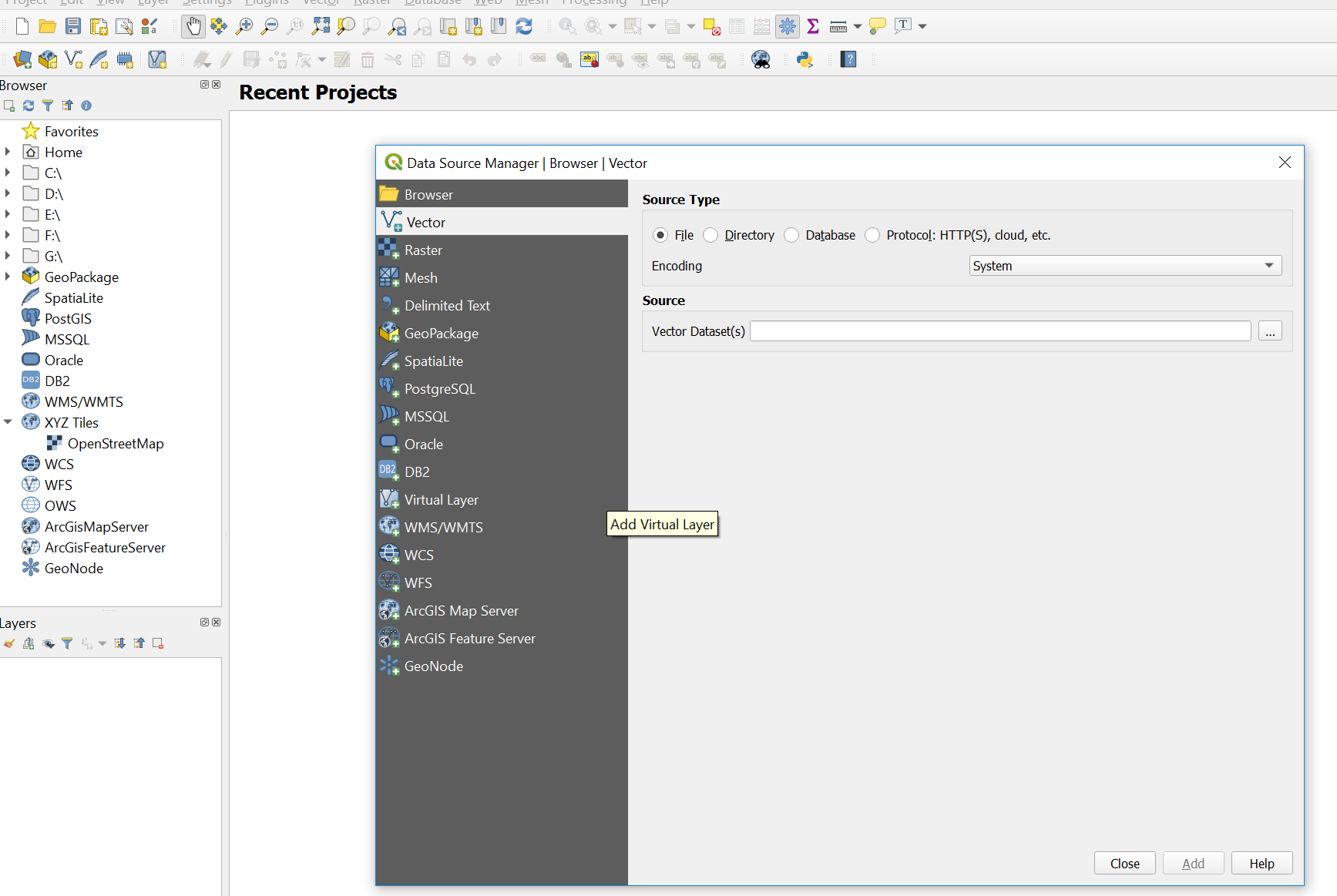
- Navigate to the London boroughs layer and add it, you then have to close the data source manager
Just like in ArcMap you can right click on the layer to view the attribute table. Unlike ArcMap you have to load the .csv file into QGIS in order to join it to a shapefile.
- Open the data source manager and select Delimited Text
- Navigate to our
.csvfile and provide a suitable layer name - Under Record and Fields Options make sure the number of header lines to discard is 0 and the First record has field names box is selected (this is assuming you left a title for each coloumn in your
.csv) - Under Geometry Definition select No geometry (attribute table only)
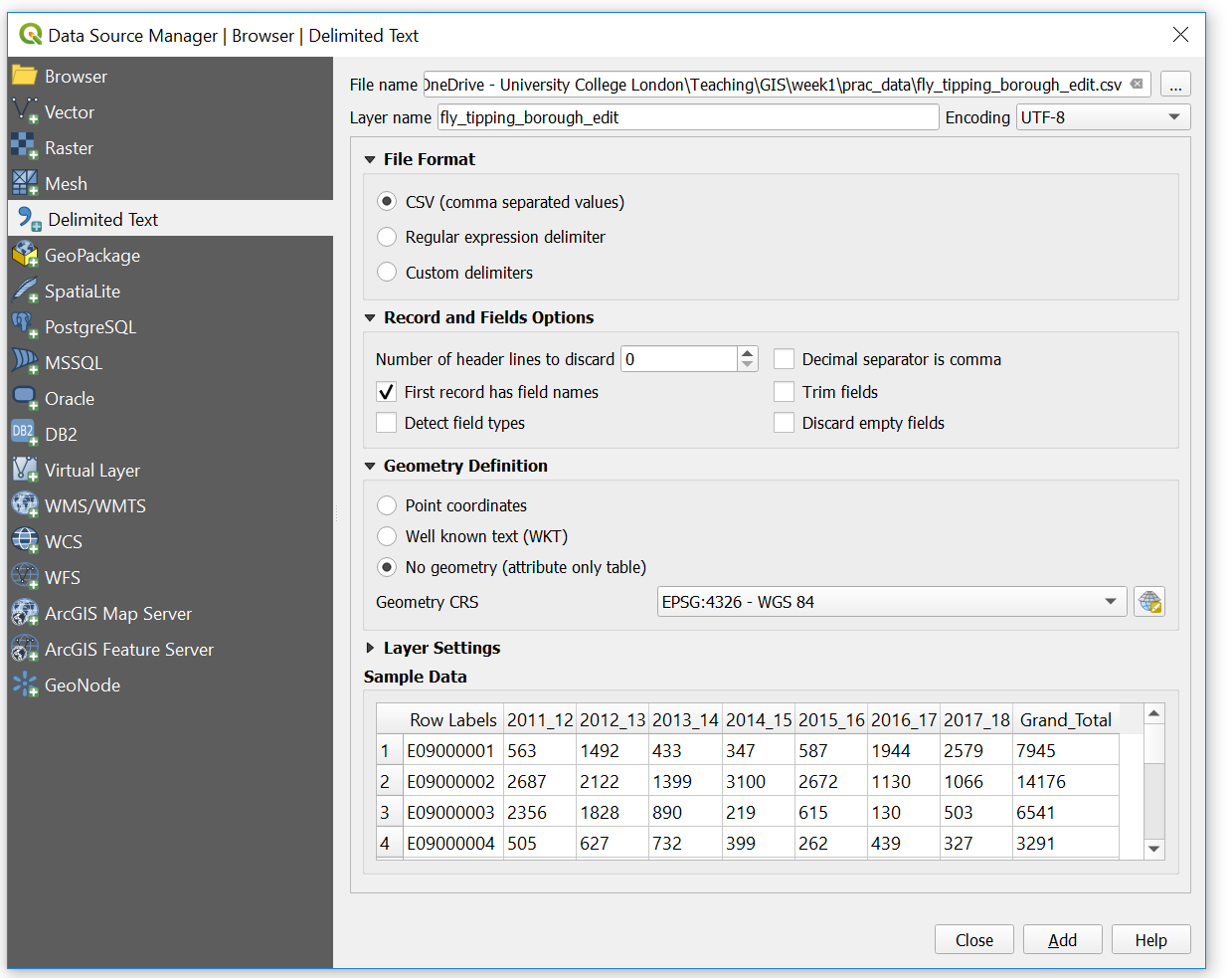
Does the sample data seem right?
- If so, click add then close.
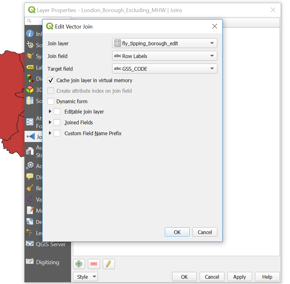
3.5.3 Join data
- Right click on the London boroughs layer > Properties > Joins
- Click the plus button at the bottom of the box
- Complete the dialouge box
3.5.4 Export data
Now instead of using a GeoDatabase, let’s export to a GeoPackage.
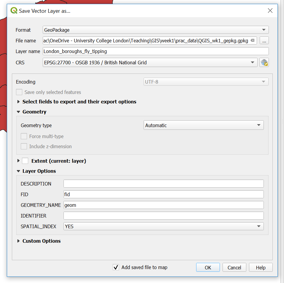
- Right click on the London boroughs layer > Export > Save Feautre As
- Select the GeoPackage format and complete the File name (the saved file name for the GeoPackage) and the Layer name (the name for this layer within the GeoPackage). Recall that a GeoPackage can store many data layers as a single file
- The new layer will be added to the map, so you can remove the old one
We’ve now made a GeoPackage that we can connect our map project to.
- Under Browser, Right click on GeoPackage > New Connection > Navigate to your GeoPackage
- Click the down arrow left to GeoPackage and you should see the one you just navigated to. Click the down arrow on the database and you can see your layer.
- Now we are going to import our
.csvinto our GeoPackage. To do so go: Database > DB Manager - Select your GeoPackage in the left hand pane
- Import layer/file then select the
.csv. Click Ok.
Again, remember that the .csv in the Layers tab (bottom left) is the original. Remove it, then from the GeoPackage just click, hold and drag the .csv into the layer pane.
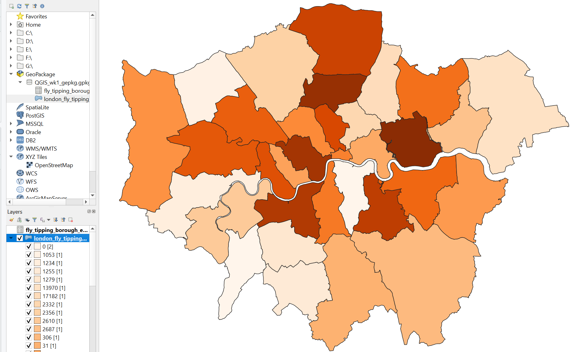
Now let’s make a quick thematic map like we did in ArcMap.
- Right click on your London boroughs layer > Properties > Symbology
- Select categorised and choose a data coloumn and color ramp
You could also select graduated, however our joined data fields are in the wrong data type. If you wish to change them follow this guide: https://wiki.tuflow.com/index.php?title=QGIS_Change_Attribute_Type
- Save your QGIS project
You should have produced something like this:
Spatial reference
QGIS is similar but different to ArcMap. QGIS defaults to the Coordiante Reference System (CRS) WGS 84, or known by its European Petroleum Survey Group (EPSG) code 4326. However, when you add your first layer in will default to that CRS.
You can change the CRS by going File > Properties and selecting CRS in the left hand pane.
3.6 R
3.6.1 Introduction
R is both a programming language and software environment, originally designed for statistical computing and graphics. R’s great strength is that it is open-source, can be used on any computer operating system and free for anyone to use and contribute to. Because of this, it is rapidly becoming the statistical language of choice for many academics and has a huge user community with people constantly contributing new packages to carry out all manner of statistical, graphical and importantly for us, geographical tasks.
The purpose of this practical is just to demostrate data loading and manipulation in different software. The next practical will provide much more detail on R, so don’t worry.
Search for and open R Studio.
You can install R Studio on your own machine from:
https://www.rstudio.com/products/rstudio/download/#download
R studio requires R which you can download from:
RStudio is a free and open-source integrated development envrionment for R - it makes R much easier to use.
In RStduio go:
- File > New File > R Script
You should be able to see these quadrants:
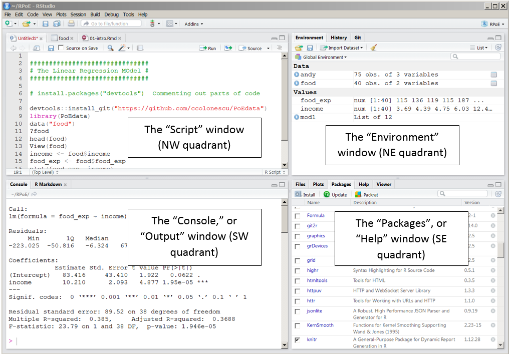
Below are bits of code, to start we will work using the console. So just copy the bits of code into the console window, changing the file names to where your data is stored. Then at the end of this section I’ll show you how to make a script.
R works on packages that are collections of functions and data. For this practical we will need the ones listed in the code chuck below. Whilst we’ve installed them, we haven’t yet loaded them. It’s best practice to do all this at the start of your code, however, for demonstration purpoposes I’ll load each one as we need it.
Packages we’ve installed:
- sf: simple features, standad way to encode spatial vector data
- tmap: layer-based and easy approach to make thematic maps
- tmaptools: set of tools for reading and processing spatial data
- RSQLite: embeds the SQLite database engine in R
Here, repos stands for repository.
3.6.2 Load data
Great, load the sf package so we can read our shapefile in - remember to change to filepath to your shapefile.
library(sf)
shape <- st_read("Prac1_data/statistical-gis-boundaries-london/ESRI/London_Borough_Excluding_MHW.shp")
## Reading layer `London_Borough_Excluding_MHW' from data source `N:\Documents\Teaching\CASA0005practicals\CASA0005\Prac1_data\statistical-gis-boundaries-london\ESRI\London_Borough_Excluding_MHW.shp' using driver `ESRI Shapefile'
## Simple feature collection with 33 features and 7 fields
## geometry type: MULTIPOLYGON
## dimension: XY
## bbox: xmin: 503568.2 ymin: 155850.8 xmax: 561957.5 ymax: 200933.9
## epsg (SRID): NA
## proj4string: +proj=tmerc +lat_0=49 +lon_0=-2 +k=0.999601272 +x_0=400000 +y_0=-100000 +datum=OSGB36 +units=m +no_defsTo get a summary of the data held within the shapefile data (attribute table) enter the following:
##                    NAME         GSS_CODE     HECTARES
##  Barking and Dagenham: 1   E09000001: 1   Min.   :  314.9
##  Barnet              : 1   E09000002: 1   1st Qu.: 2724.9
##  Bexley              : 1   E09000003: 1   Median : 3857.8
##  Brent               : 1   E09000004: 1   Mean   : 4832.4
##  Bromley             : 1   E09000005: 1   3rd Qu.: 5658.5
##  Camden              : 1   E09000006: 1   Max.   :15013.5
##  (Other)             :27   (Other)  :27
##    NONLD_AREA     ONS_INNER SUB_2009  SUB_2006           geometry
##  Min.   :  0.00   F:19      NA's:33   NA's:33   MULTIPOLYGON :33
##  1st Qu.:  0.00   T:14                          epsg:NA      : 0
##  Median :  2.30                                 +proj=tmer...: 0
##  Mean   : 64.22
##  3rd Qu.: 95.60
##  Max.   :370.62
##
To have a quick look what the shapefile looks like enter the following:
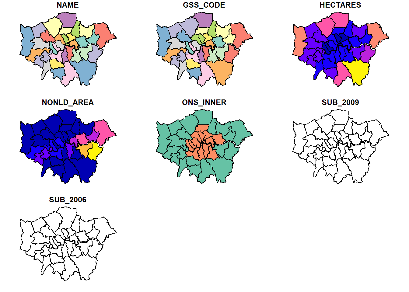
From what we did in QGIS and ArcMap this should look familiar.
We now need to load our .csv file:
To view the data just input:
##     Row.Labels X2011_12 X2012_13 X2013_14 X2014_15 X2015_16 X2016_17
## 1    E09000001      563     1492      433      347      587     1944
## 2    E09000002     2687     2122     1399     3100     2672     1130
## 3    E09000003     2356     1828      890      219      615      130
## 4    E09000004      505      627      732      399      262      439
## 5    E09000005     6713     2232     3189     3926     3980     4366
## 6    E09000006      306      479      653      462      326      228
## 7    E09000007     5541     5962     8281     4837     4719     4656
## 8    E09000008       31      108      460      712     1707      637
## 9    E09000009     6727     5679     6543     5521     6067    12688
## 10   E09000010     7262     3595     3269     4937     5292    10894
## 11   E09000011     6344     7482    13950    17667     6410     2188
## 12   E09000012     2332     1456    10495     8865     9494     5601
## 13   E09000013     6944     1719     1719     1632     1868     4857
## 14   E09000014     8817     4719     7633     8639     3615     5131
## 15   E09000015     1053        0        0      995     1354     1385
## 16   E09000016    13970    13762    13393     7404     8523    11748
## 17   E09000017     5120     4188     3101        0      620     3031
## 18   E09000018     1234     1030      994     2190     1865     2242
## 19   E09000019     6959     6167     8646     8172     8250     7878
## 20   E09000020     4773     5009     6353     6651     6308     9282
## 21   E09000021        0        0        0        0        0        0
## 22   E09000022      598        0        0        0        0        0
## 23   E09000023      789     1083     1499     2627     2611     1454
## 24   E09000024     1279     1299     1305     6985     2542     6056
## 25   E09000025     9593     7283    10354     8620    10621     5155
## 26   E09000026     6114     6913     4778     6306     4319     2489
## 27   E09000027     2610     2291     2647      207     2133     3337
## 28   E09000028        0     1194     3776     1889     1476     1937
## 29   E09000029     1255      201      755      545      146      278
## 30   E09000030     3251     4909    18057    17064    17494    14601
## 31   E09000031    17182    17049    17176    17361    12290    18459
## 32   E09000032     8226     5166     6674     4977     8547     9582
## 33   E09000033     8367     6636     6166     6380     3447     3876
## 34 Grand Total   149501   123680   165320   159636   140160   157679
##    X2017_18 Grand_Total
## 1      2579        7945
## 2      1066       14176
## 3       503        6541
## 4       327        3291
## 5      7483       31889
## 6       258        2712
## 7     12671       46667
## 8      2684        6339
## 9      5471       48696
## 10     5855       41104
## 11     1443       55484
## 12    11172       49415
## 13     2982       21721
## 14     3171       41725
## 15     1622        6409
## 16    10463       79263
## 17     4393       20453
## 18     4334       13889
## 19     7231       53303
## 20    10165       48541
## 21        3           3
## 22      959        1557
## 23     1330       11393
## 24     6299       25765
## 25     3615       55241
## 26     5670       36589
## 27     2615       15840
## 28     2255       12527
## 29      450        3630
## 30    13316       88692
## 31    17036      116553
## 32     9735       52907
## 33     7111       41983
## 34   166267     1062243
3.6.3 Join data
In R we’ve given our London boroughs shapefile the name shape and our flytipping .csv the name mycsv. If you look in the Environment quadrant you should see them both listed.
Join the .csv to the shapefile. Here, replace Row.Labels with whatever your GSS_CODE is called in the .csv:
library(tmap)
library(tmaptools)
shape<-append_data(shape, mycsv, key.shp="GSS_CODE", key.data = "Row.Labels")
## Over coverage: 1 out of 34 data records were not appended. Run over_coverage() to get the corresponding data row numbers and key values.Let’s break this down a bit. We just created a data frame that is a table has a variable and each row contains a set of values - so a normal table. The match simply found the GSS_CODE values in the .csv and joined the data.
The message detailing 1 out of the 34 data records were not appended refers to the Grand Total row within the .csv.
Check the merge was successful, this is just going to show the top 10 rows:
## Simple feature collection with 10 features and 15 fields
## geometry type:  MULTIPOLYGON
## dimension:      XY
## bbox:           xmin: 503568.2 ymin: 155850.8 xmax: 561957.5 ymax: 198355.2
## epsg (SRID):    NA
## proj4string:    +proj=tmerc +lat_0=49 +lon_0=-2 +k=0.999601272 +x_0=400000 +y_0=-100000 +ellps=airy +towgs84=446.448,-125.157,542.06,0.1502,0.247,0.8421,-20.4894 +units=m +no_defs
##                    NAME  GSS_CODE  HECTARES NONLD_AREA ONS_INNER SUB_2009
## 21 Kingston upon Thames E09000021  3726.117      0.000         F     <NA>
## 8               Croydon E09000008  8649.441      0.000         F     <NA>
## 6               Bromley E09000006 15013.487      0.000         F     <NA>
## 18             Hounslow E09000018  5658.541     60.755         F     <NA>
## 9                Ealing E09000009  5554.428      0.000         F     <NA>
## 16             Havering E09000016 11445.735    210.763         F     <NA>
## 17           Hillingdon E09000017 11570.063      0.000         F     <NA>
## 15               Harrow E09000015  5046.330      0.000         F     <NA>
## 5                 Brent E09000005  4323.270      0.000         F     <NA>
## 3                Barnet E09000003  8674.837      0.000         F     <NA>
##    SUB_2006 X2011_12 X2012_13 X2013_14 X2014_15 X2015_16 X2016_17 X2017_18
## 21     <NA>        0        0        0        0        0        0        3
## 8      <NA>       31      108      460      712     1707      637     2684
## 6      <NA>      306      479      653      462      326      228      258
## 18     <NA>     1234     1030      994     2190     1865     2242     4334
## 9      <NA>     6727     5679     6543     5521     6067    12688     5471
## 16     <NA>    13970    13762    13393     7404     8523    11748    10463
## 17     <NA>     5120     4188     3101        0      620     3031     4393
## 15     <NA>     1053        0        0      995     1354     1385     1622
## 5      <NA>     6713     2232     3189     3926     3980     4366     7483
## 3      <NA>     2356     1828      890      219      615      130      503
##    Grand_Total                       geometry
## 21           3 MULTIPOLYGON (((516401.6 16...
## 8         6339 MULTIPOLYGON (((535009.2 15...
## 6         2712 MULTIPOLYGON (((540373.6 15...
## 18       13889 MULTIPOLYGON (((521975.8 17...
## 9        48696 MULTIPOLYGON (((510253.5 18...
## 16       79263 MULTIPOLYGON (((549893.9 18...
## 17       20453 MULTIPOLYGON (((510599.8 19...
## 15        6409 MULTIPOLYGON (((510599.8 19...
## 5        31889 MULTIPOLYGON (((525201 1825...
## 3         6541 MULTIPOLYGON (((524579.9 19...
Now, let’s make a quick thematic map (or a qtm) using the package tmap. I’ve made mine for flytipping between 2011 and 2012 (coloumn X2011_12):
## tmap mode set to plotting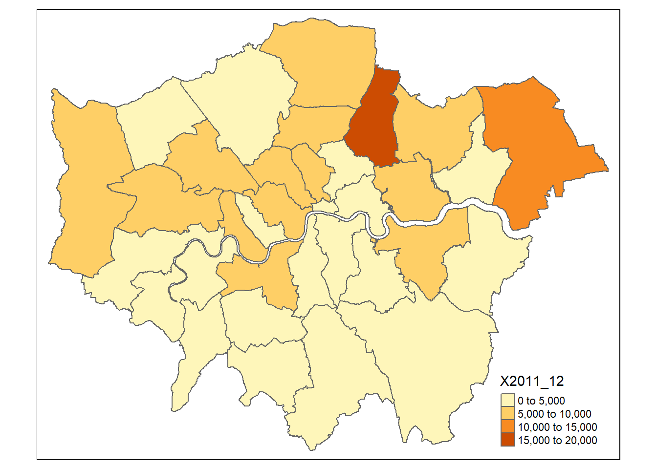
3.6.4 Export data
Finally write shape to a new GeoPackage (.gpkg) giving it the layer name of your choice:
## Deleting layer `london_boroughs_fly_tippint' using driver `GPKG'
## Updating layer `london_boroughs_fly_tippint' to data source `Prac1_data/Rwk1.gpkg' using driver `GPKG'
## features:       33
## fields:         15
## geometry type:  Multi Polygon
Let’s also add the .csv as we did in QGIS. This is a bit more complicated as we have to use the SQLite datavase package.Firstly, connect to the .gpkg we just made:
Now examine what is in the .gpkg:
##  [1] "gpkg_contents"
##  [2] "gpkg_extensions"
##  [3] "gpkg_geometry_columns"
##  [4] "gpkg_metadata"
##  [5] "gpkg_metadata_reference"
##  [6] "gpkg_ogr_contents"
##  [7] "gpkg_spatial_ref_sys"
##  [8] "gpkg_tile_matrix"
##  [9] "gpkg_tile_matrix_set"
## [10] "london_boroughs_fly_tippint"
## [11] "original_csv"
## [12] "rtree_london_boroughs_fly_tippint_geom"
## [13] "rtree_london_boroughs_fly_tippint_geom_node"
## [14] "rtree_london_boroughs_fly_tippint_geom_parent"
## [15] "rtree_london_boroughs_fly_tippint_geom_rowid"
## [16] "sqlite_sequence"
Then add add our .csv and disconnect from the .gpkg:
3.6.5 Making a script
To convert this bit of analysis into a script that we could save and run again in future, I would write the following in the script quadrant:
install.packages("sf", "tmap", "tmaptools", "RSQLite", repos = "https://www.stats.bris.ac.uk/R/")
library(sf, tmap, tmaptools, RSQLite)
shape <- st_read("Prac1_data/statistical-gis-boundaries-london/ESRI/London_Borough_Excluding_MHW.shp")
mycsv = read.csv("Prac1_data/fly_tipping_borough_edit.csv")
shape<-append_data(shape, mycsv, key.shp="GSS_CODE", key.data = "Row.Labels")
tmap_mode("plot")
qtm(shape, fill = "X2011_12")
st_write(shape, "Prac1_data/Rwk1.gpkg", "london_boroughs_fly_tippint", delete_layer=TRUE)
con = dbConnect(SQLite(),dbname="Prac1_data/Rwk1.gpkg")
dbListTables(con)
dbWriteTable(con,"original_csv", mycsv, overwrite=TRUE)
dbDisconnect(con)You can then save your script through File > Save As
When the code is laid out like this you’ll notice a lot of repetition, for example i’ve repeated similar file path names three times. This is very messy code which we will address in future practicals.
3.7 What will I use
Well… it depends. If you wanted to quickly open a dataset to explore its contents then i’d use QGIS or ArcMap. However, if you had 100 raster images that you wanted to clip to your study area, i’d automate it in R. There are also specfic packages developed for each type of software that might dictate what you use, for example I recently made use of the Urban Multi-sacle Envrionmental Predictor (UMEP) plugin in QGIS. That said, as I needed to match different hourly meterological varaibles over a three year period I automated the first part of the analysis in R and loaded a .csv into QGIS.
4 Data sources and task
Below i’ve listed a few good data sources. For this week’s task explore these and any others you can find and get an interesting dataset (e.g. in this practical our flytipping .csv) that you could join to some spatial data (e.g. in this practical the London boroughs .shp). This could be for any location in the world.
4.1 UK Data Service
The UK Data Service geography service (https://census.edina.ac.uk/) has a library of hundreds of current and former boundary datasets for which attribute data are produced in the UK.
4.2 ONS
The Office for National Statistics (ONS) are the national statistical agency for England and Wales and have recently started to provide access to boundary data for the statistics they produce for various geographic areas.
Many of the boundaries on the ONS Geoportal are also available from the Edina Census Geography website in a more flexible fashion, however the ONS website provides very quick access to bulk-downloads – something which can be very useful when reading data directly from the web using computer software.
4.3 OS
The Ordnance Survey (OS) are the national mapping agency for the UK. A few years ago, they opened up a number of their data products for public use including greenspace, OS Open Map and OS Terrain.
For the full range see: https://www.ordnancesurvey.co.uk/business-and-government/products/finder.html?Licensed%20for=OpenData%20(Free)&withdrawn=on
4.4 Edina Digimap
Before the Ordnance Survey opened up much of its data for public use, academics and students in the UK could access OS data using the Edina Digimap Service – this service is still available today and provides access to a number of products in addition to those available from OS Open Data.
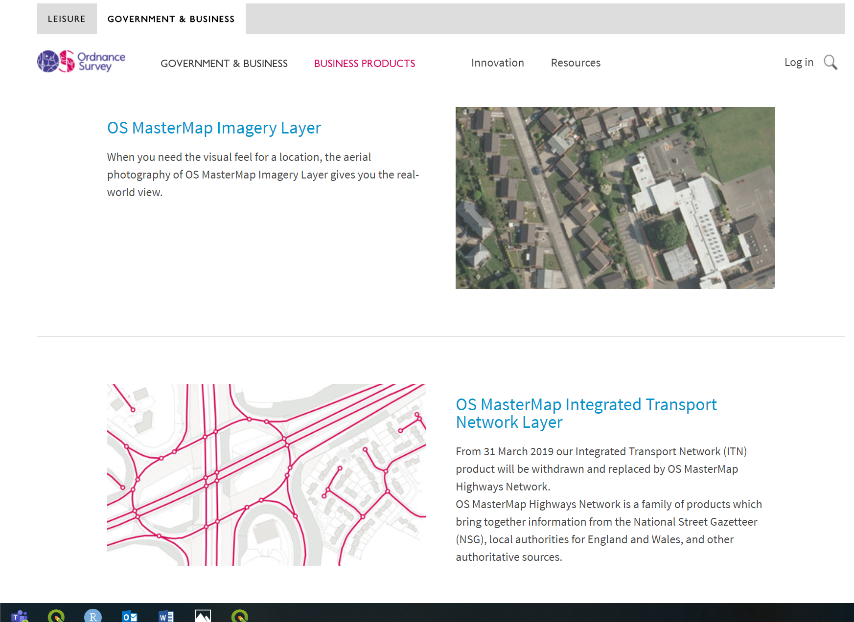
Perhaps the most exciting of the additional OS data products available from Digimap is OS MasterMap. MasterMap is a framework for all OS data and contains layers of data that include details of real world objects such as buildings, roads, paths, rivers, physical structures and land parcels, as well as the complete UK transport network. Whilst we still are required to go through Edina OS have recently annonced plans to make this dataset free in the near future under the new Geospatial Commission.
4.5 OSM
Open Street Map (OSM) is a fantastic resource – as the name suggests, all data contained in Open Street Map are open and free for anyone to use. Much like Wikipedia, anyone can contribute content to OSM and this brings with it its own benefits (frequent updates, very large user-base) and problems (data quality and patch coverage). OSM is a very good example of Volunteered Geographic Information (VGI).
It’s possible to download OSM data straight from the website, although the interface can be a little unreliable (it works better for small areas). There are, however, a number of websites that allow OSM data to be downloaded more easily and are directly linked to from the ‘Export’ option in OSM. Geofabrik (https://www.geofabrik.de/data/download.html) allows you to download frequently updated Shapefiles for various global subdivisions.
4.6 DEFRA
The Department for Environmen and Rural Affairs (DEFRA) have recently created the Data Services Platform to openly distribute envrionmental data. See: https://environment.data.gov.uk/
4.7 Data lists
Another good place to start searching for data are data lists. They simply provide a comprehensive overview of all available data conveniently categorised by discipline and country.
I normally use this one: https://freegisdata.rtwilson.com/
5 Summary
Within this practical we have explored the different types, formats and software used to store, analyse and manipulate spatial data. In relfecting upon this practical you should consider the (dis)advtanges of each, where and when they might be approraite and the overall practicality. Next week we will delve further into R and RStudio.